Constructing and challenging component graphs

By UK GCSE Physics · independent study · myAudience

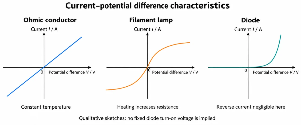
Image: illustration, not a documentary photograph. Original myAudience teaching concept; generated raster independently inspected. · Original generated teaching illustration; source facts attributed in the lesson.

Constructing and challenging component graphs

Start with the axes, units and collected range. Plate 04 is a shape comparison with no numerical scales: it cannot supply a tangent value or rank the absolute resistances of its different panels. On paper plot original paired readings on regular scales using most of the space, including zero and negative regions when sampled. Draw a best-fit straight line for a justified linear model or a smooth curve for a non-linear one. Connecting every noisy point creates artificial changes of slope.

For an I–V straight line, gradient is change in I divided by change in V, with units A/V. Only a through-origin line has I/V equal to its constant gradient. On a V–I graph the slope instead has units V/A and represents resistance for an ohmic line through zero. State the axis order before interpreting steepness. A straight line with an intercept may signal an offset or a different model; it does not establish direct proportionality.

At a point on a curved I–V graph, ordinary operating resistance is V/I. A tangent measures the local change in current per change in potential difference; choose widely separated points on the drawn tangent, not neighbouring noisy curve samples. The reciprocal of that tangent slope is a small-change resistance, a distinct extension used here to expose a common error. Do not present it as the required operating resistance. Your own tangent drawing and scale reading will introduce estimation uncertainty.

Plate 05 uses different variables: resistance against temperature or illumination. Its declining slope is not electrical conductance, and the unnumbered curves do not specify a threshold. For an LDR test, hold temperature and geometry comparable and record actual illumination if claiming a calibrated light-intensity graph. Distance from a lamp alone does not measure intensity. For an NTC test, allow temperature to settle and limit self-heating; otherwise the measurement itself changes the sensor condition.

Use plate 06 to collect matched test-component V and I. Choose smaller steps where a diode forward curve changes rapidly, retain a suitable series protection resistor, and respect approved ratings. Reverse readings below resolution should be reported as not resolved. Do not draw an exactly zero physical leakage or invent breakdown data. For a resistor, compare repeats at the same V before and after the sweep to assess drift. Similar shapes cannot prove good temperature control or apparatus competence.

Vocabulary: secant = line through two curve points; tangent = local-direction line at a curve point; intercept = value where the graph meets an axis; operating resistance = V/I at a specified point; not resolved = below measurement capability.

Worked example: An invented constant-temperature resistor dataset is (V, I): (−4.0, −0.20), (−2.0, −0.10), (0, 0), (2.0, 0.10), (4.0, 0.20), in V and A. Construct axes and infer resistance. Separately a lamp passes through (4.0 V, 0.40 A), with a supplied tangent through (2.0 V, 0.32 A) and (6.0 V, 0.48 A). Calculate its operating resistance and explain the tangent.

For the resistor, a regular V scale from −4 to +4 V and I scale from −0.20 to +0.20 A includes all five points. Plot and fit through the origin; gradient = (0.20 − (−0.20))/(4.0 − (−4.0)) = 0.050 A/V.

R = 1/0.050 = 20 Ω. Swapping axes gives a V–I slope of 20 V/A = 20 Ω. Keep these conclusions conditional on constant temperature and the invented exact data.

Lamp operating R = 4.0/0.40 = 10 Ω. Tangent slope = (0.48 − 0.32)/(6.0 − 2.0) = 0.040 A/V. Its reciprocal is 25 Ω, not the operating 10 Ω.

The tangent predicts a local approximate increase 0.040 × 0.20 = 0.0080 A for a small 0.20 V increase. Do not extend this local approximation across the entire lamp curve.

Answer: Resistor 20 Ω; lamp operating resistance 10 Ω; tangent slope 0.040 A/V and reciprocal 25 Ω, a different small-change quantity.

Check your understanding: A measured straight line follows I = 0.050V + 0.010, using A and V. Is it directly proportional? At 2.0 V calculate V/I. Would forcing the fit through zero fix the evidence?

Answer: No; at 2.0 V, I = 0.110 A and V/I = 18.1818… Ω (about 18 Ω to two significant figures). Forcing zero hides the offset.

Why: At V = 0 the model gives 0.010 A, so I/V is not constant. The slope alone does not equal I/V here. Check meter zero, paired readings and model assumptions; do not erase the intercept to recover the expected answer.