Expressing uncertainty without claiming certainty

By UK A Level Physics · independent study · myAudience

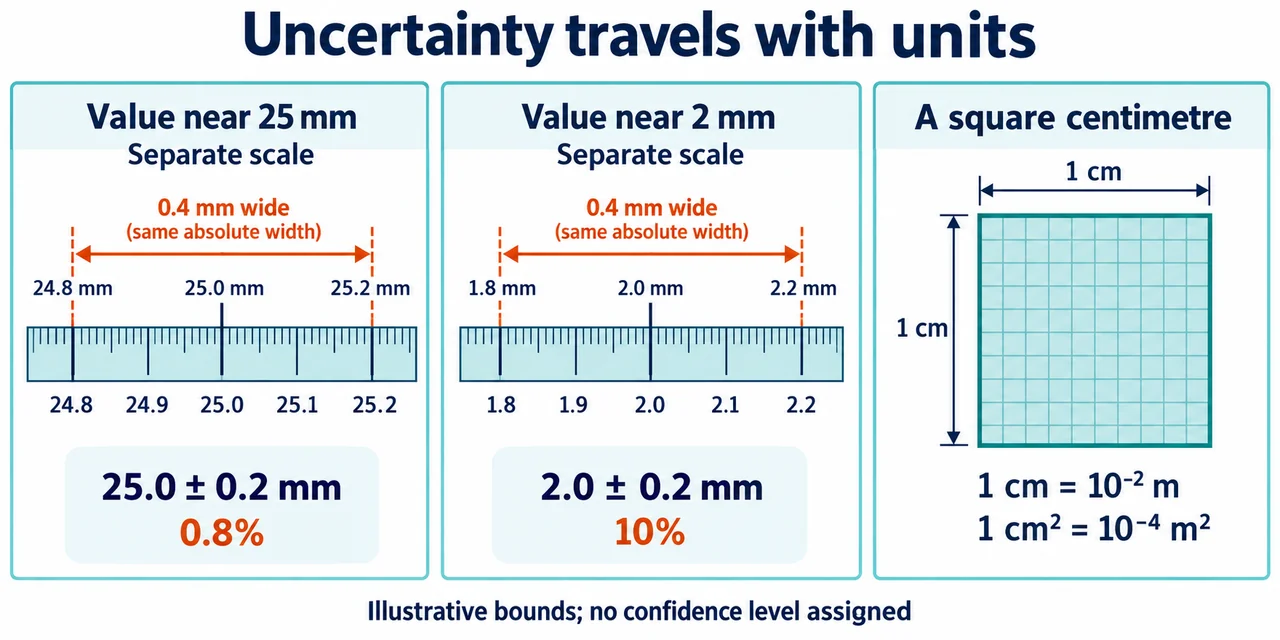
Image: illustration, not a documentary photograph. Original teaching model created for myAudience. · Original generated teaching illustration; no board endorsement or source textbook artwork reproduced.

Expressing uncertainty without claiming certainty

Uncertainty describes the range of values reasonably attributed to a measured quantity; error is the difference between a measured value and a reference value. Because the true value is usually unknown, the actual error need not be known even when an uncertainty has been estimated. This lesson assumes means, subtraction and percentages. Vocabulary includes absolute uncertainty, fractional uncertainty, percentage uncertainty and significant figures.

For an illustrative repeated-length dataset of 24.8, 25.0, 25.2 and 25.0 mm, the mean is 25.0 mm and the half-range is (25.2 − 24.8)/2 = 0.2 mm. Reporting 25.0 ± 0.2 mm is a simple school estimate of scatter, with the method stated. Half-range is not automatically a confidence interval, and a small sample may miss larger variations. Instrument resolution, calibration and method must also be considered; the spread alone cannot detect a constant zero offset.

Absolute uncertainty has the same unit as the quantity. Fractional uncertainty is Δx/|x|, and percentage uncertainty is 100Δx/|x|. Here they are 0.2/25.0 = 0.008 and 0.8%. The same absolute uncertainty matters more for a small measurement: ±0.2 mm on 2.0 mm is 10%. The fraction is undefined for a nominal value of zero, so do not force this formula onto a zero crossing; use an absolute interval instead.

Resolution gives evidence for an uncertainty estimate, not a universal rule. A rounding-only model for an analogue reading may assign half a scale division; a digital instrument's specified accuracy can exceed one final digit. When taking a difference between two ruler readings, both endpoints contribute. State the convention or manufacturer information used. If the illustrative uncertainty is quoted to one significant figure, give the value to the same decimal place: 25.0 ± 0.2 mm, not 25.00000 ± 0.2 mm.

NIST distinguishes uncertainty components assessed statistically from those assessed by other information. Those categories are not identical to 'random' and 'systematic'. At this stage, the important habit is to identify the source of each component and explain what the stated interval means. A calculated mean with extra calculator digits is not extra knowledge. Report a justified result, preserve raw data, and explain limitations so another reader can judge the measurement honestly.

Read the two rulers separately. The endpoints are 24.8 and 25.2 mm in the first panel and 1.8 and 2.2 mm in the second. In each case the full interval is 0.4 mm wide, whereas the absolute uncertainty is its half-width, 0.2 mm. The percentages compare that half-width with the central value: 100(0.2/25.0) = 0.8% and 100(0.2/2.0) = 10%. The larger percentage does not mean the second interval is physically wider. It means the stipulated bound is large relative to the quantity being reported. Separate scales prevent the drawings from implying that the two objects themselves have equal length.

The area panel requires two length conversions, one for each side. A square with sides 1 cm and 1 cm has area (0.01 m)(0.01 m) = 0.0001 m². The grid is schematic, not a calibrated photograph. A prefix acts on the unit before the unit is squared: cm² means (cm)². Converting a stated uncertainty to another unit requires the same factor as the central value. Thus 25.0 ± 0.2 mm becomes 0.0250 ± 0.0002 m; its percentage uncertainty stays 0.8%. A change of units cannot improve precision.

**Worked subtraction and addition.** Two independently bounded position readings are x₁ = 12.4 ± 0.3 cm and x₂ = 28.6 ± 0.4 cm. Find the displacement and its conservative bound. The centre is 16.2 cm. The lowest difference is 28.2 − 12.7 = 15.5 cm; the highest is 29.0 − 12.1 = 16.9 cm. Therefore report 16.2 ± 0.7 cm. Adding the positions instead gives 41.0 ± 0.7 cm. For sums and differences the absolute contributions add under this worst-case bound convention; subtracting the central values does not subtract their uncertainties.

**Worked multiplication with exact endpoint check.** Let a = 20.0 ± 0.2 mm and b = 10.0 ± 0.1 mm be independently bounded positive lengths. The central area is 200 mm². First-order fractional propagation gives 0.2/20 + 0.1/10 = 0.02, hence approximately 200 ± 4 mm². Exact endpoint products are 19.8×9.9 = 196.02 and 20.2×10.1 = 204.02 mm². The asymmetry exposes the discarded product of small errors; it does not invalidate the useful first-order approximation. An exact enclosing interval is [196.02, 204.02] mm². In SI the first-order report is 0.000200 ± 0.000004 m², not 0.0200 m². This is a bound calculation, not a standard deviation or a 95% interval.

**Transfer check.** A zero offset z is common to both readings, so x₁ = r₁ − z and x₂ = r₂ − z. Does the uncertainty in z contribute twice to x₂ − x₁? Explain algebraically before calculating. Answer: (r₂ − z) − (r₁ − z) = r₂ − r₁, so this exactly shared additive offset cancels. Treating it as two independent contributions would discard known correlation. Scale-factor errors do not generally cancel from a difference. School propagation rules need an explicit measurement model; they are not universal statistical rules.

**All-prefix independent practice.** Convert to SI and normalised standard form: 2.4 THz; 3.6 GHz; 7.2 MJ; 5.0 kV; 8.1 cm; 4.3 mm; 6.2 μA; 9.4 nm; 1.7 pF; 2.8 fs. Answers in order: 2.4×10¹² Hz, 3.6×10⁹ Hz, 7.2×10⁶ J, 5.0×10³ V, 8.1×10⁻² m, 4.3×10⁻³ m, 6.2×10⁻⁶ A, 9.4×10⁻⁹ m, 1.7×10⁻¹² F, 2.8×10⁻¹⁵ s. These are the ten prefixed symbols T, G, M, k, c, m, μ, n, p and f required here. A separate unprefixed case is 0.0065 s = 6.5×10⁻³ s. Convert 3.0 mm³ too: 3.0×10⁻⁹ m³. Confusing milli with mega changes a value by a factor of 10⁹.

Worked example: For 24.8, 25.0, 25.2 and 25.0 mm, calculate the mean, half-range and percentage uncertainty.

Mean = (24.8 + 25.0 + 25.2 + 25.0)/4 = 25.0 mm.

Half-range = (25.2 − 24.8)/2 = 0.2 mm.

Percentage = 100 × 0.2/25.0 = 0.8%.

Answer: 25.0 ± 0.2 mm; 0.8%, using half-range as the stated illustrative convention.

Check your understanding: A constant 0.4 mm zero offset is present. Does a 0.2 mm half-range prove accuracy?

Answer: No. Correct or investigate the offset and retain an uncertainty for that correction.

Why: The repeats describe scatter; a shared shift can leave that scatter unchanged while moving every result.