Error bars, gradients and intercepts

By UK A Level Physics · independent study · myAudience

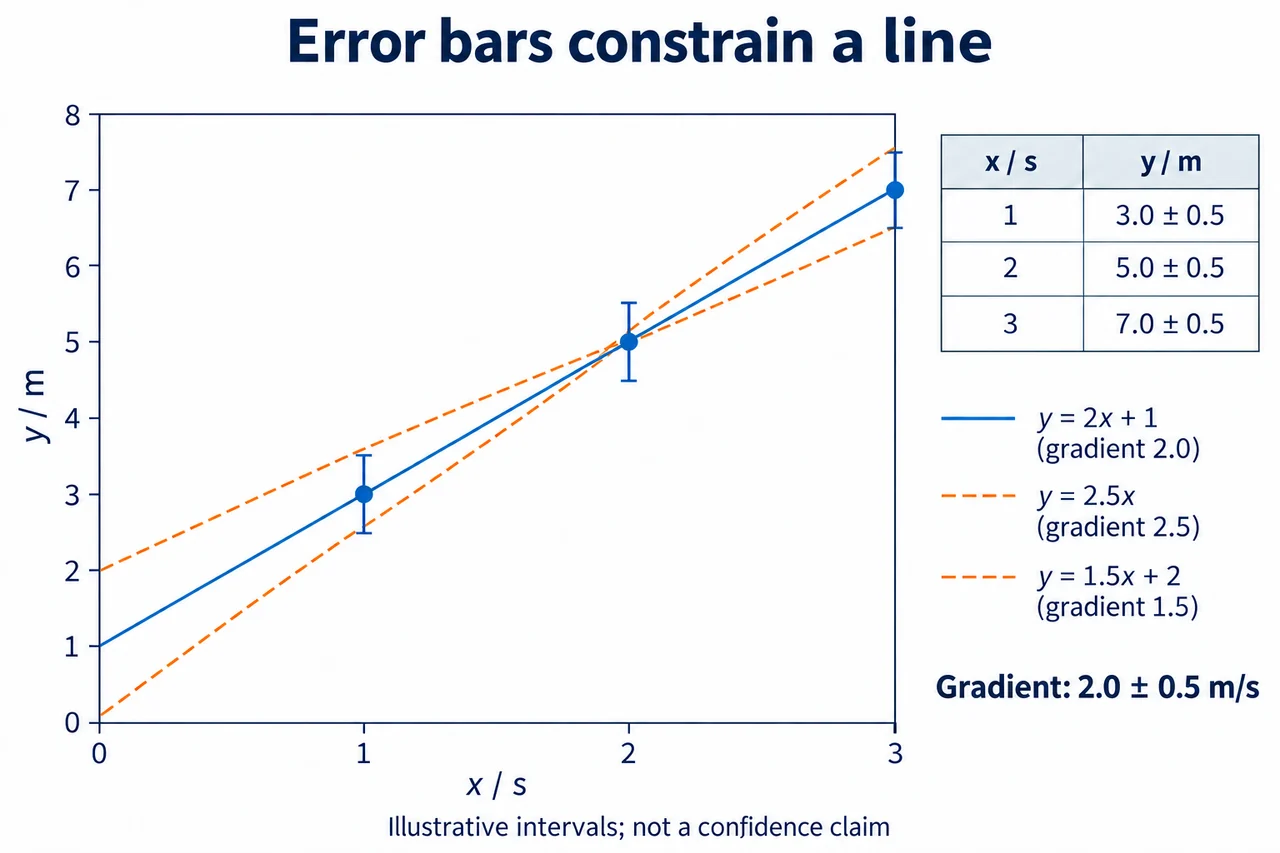
Image: illustration, not a documentary photograph. Original teaching model created for myAudience. · Original generated teaching illustration; no board endorsement or source textbook artwork reproduced.

Error bars, gradients and intercepts

A graph combines a physical model with measurement evidence. This lesson assumes straight-line algebra and uncertainty intervals. Label each axis with the quantity and unit, choose a scale that uses the available area, and plot points without joining every neighbouring point. For y = mx + c, m describes change in y per change in x, while c is the y-value extrapolated to x = 0. Their units need not match: y in metres and x in seconds gives m in m s⁻¹ and c in metres.

An error bar represents the interval assigned to a plotted coordinate. If only y is uncertain, draw a vertical bar; if x is also uncertain, include its horizontal interval. Explain whether the bars represent estimated bounds or another uncertainty convention. A line of best fit should describe the overall trend rather than pass through every central point. If no straight line is consistent with the intervals, investigate a curved relationship, underestimated uncertainty or a systematic effect rather than forcing agreement.

For an original illustrative dataset x = 1, 2, 3 s and y = 3.0, 5.0, 7.0 m, with ±0.5 m at each y and negligible x uncertainty, the central line is y = 2x + 1. The steepest acceptable line is y = 2.5x and the shallowest is y = 1.5x + 2. Both pass through the middle point and the allowed intervals of the endpoints. Check all intervals, not only the first and last; an interior point can rule out an endpoint-based line in another dataset.

The limiting gradients give Δm = (2.5 − 1.5)/2 = 0.5 m s⁻¹ about the central 2.0 m s⁻¹. Their intercepts span 0 to 2 m, giving c = 1 ± 1 m for these particular bounds. Gradient and intercept are related: changing the slope changes where the line crosses the axis. They are not independent adjustable errors. Use large triangles on the drawn lines, rather than adjacent noisy points, to calculate gradients accurately.

When individual error bars are absent, estimate a reasonable steepest and shallowest fit using scatter and the stated method; do not invent precise bounds unsupported by data. Extrapolating an intercept far beyond the measured x-range is especially uncertain. A nonzero intercept can suggest an offset, but does not by itself identify its cause. This graphical exercise prepares data analysis; the dataset is synthetic and neither a real measurement nor a statistical confidence claim.

**Original synthetic dataset:** exact teaching times t/s = 0,1,2,3,4; positions x/m = 0.2,2.1,4.2,6.1,8.4. No individual instrument uncertainty or confidence level is supplied. Fit x = vt + c with an intercept, rather than forcing the origin. The means are t̄ = 2 s and x̄ = 4.2 m. The least-squares slope is Σ[(t−t̄)(x−x̄)]/Σ(t−t̄)² = 20.4/10 = 2.04 m/s and c = 0.12 m. Predicted positions are 0.12,2.16,4.20,6.24,8.28 m; residuals are +0.08,−0.06,0,−0.14,+0.12 m. Their sum is zero, as expected for this intercept fit. The residual sum of squares is 0.044 m².

**Demanding check.** A learner calls the smallest and largest pairwise slopes, 1.9 and 2.3 m/s, a confidence interval. Identify two flaws and propose what can honestly be reported. Answer: selecting pairs does not define a statistical confidence procedure; the task gives no instrument model, independence evidence or population sampling model. Report the fitted slope and residual pattern, and distinguish exploratory sensitivity from quantified uncertainty. If one deliberately assumes exact t, independent constant-variance zero-mean errors in x and a correct linear model, the residual standard deviation is √(0.044/3) = 0.1211 m and the conditional standard error of slope is 0.1211/√10 = 0.03830 m/s. These are model-dependent estimates, not established properties of an experiment. No confidence interval is asserted here. A curved residual pattern or an uncertain time axis would require revisiting the model.

For a graphical answer draw a line through the overall trend, use widely separated points on that line to calculate the gradient, identify the intercept and discuss scatter. Do not join successive data points and call every segment a speed estimate of equal evidential quality. Repeating data would help investigate variation, while calibration and timing checks would investigate separate systematic effects. This exercise prepares interpretation; it is not evidence that any apparatus was used.

Worked example: Use the three synthetic points and intervals in the text to find the limiting gradients and intercepts.

Steep line: (7.5 − 2.5)/(3 − 1) = 2.5 m s⁻¹, c = 2.5 − 2.5 × 1 = 0 m.

Shallow line: (6.5 − 3.5)/2 = 1.5 m s⁻¹, c = 3.5 − 1.5 = 2 m.

At x = 2 both predict 5 m, inside the middle interval. Half-ranges are 0.5 m s⁻¹ and 1 m.

Answer: m = 2.0 ± 0.5 m s⁻¹ and c = 1 ± 1 m, with the specified illustrative bounds.

Check your understanding: Can an endpoint line be accepted if it misses the middle point’s error bar?

Answer: No.

Why: A compatible line must be consistent with every assigned interval; endpoints alone do not establish compatibility.