Demand: effective willingness, movements and shifts
By UK A Level Economics · independent study · myAudience
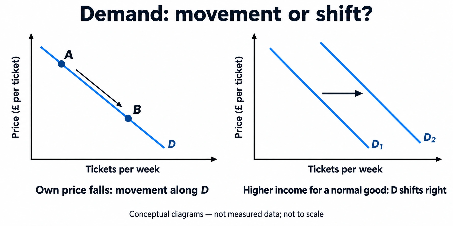
Original teaching plate generated using the built-in imagegen tool, 2026-10-04; conceptual or hypothetical, not empirical evidence. · Original generated artwork; provenance and rights acceptance pending independent review before public publication.
Demand: effective willingness, movements and shifts
Demand is willingness and ability to purchase quantities at alternative prices over a specified period. Wanting a ticket without the means to pay is not effective market demand. Define the market: cinema tickets in one town per week are not all entertainment expenditure nationally. Holding other influences constant, a lower own price usually increases quantity demanded. The demand curve places price per ticket vertically and tickets per week horizontally. A single point is quantity demanded at one price; the whole curve is the relationship. A fall in the ticket's own price causes a movement along a fixed curve, not a rightward shift of that curve.
A demand shift means quantity demanded changes at every given own price because something else changes. Income, wealth, preferences, population, expectations and prices of related goods can matter. Higher income shifts demand right for a normal good and left for an inferior good; those labels describe observed income responses, not quality or moral worth. A substitute satisfies a similar use, so a rise in its price can increase demand for this good. A complement is used with it, so a rise in that price can reduce demand. State the relationship and the relevant market instead of drawing every price change as a shift.
The plate distinguishes an A-to-B own-price movement from a D1-to-D2 shift caused by higher income for a normal good. No numerical ticks are given, and the two panels do not estimate a real income elasticity. Use its logic, then calculate from the hypothetical schedule below. A lower own price can make purchasing more attractive relative to alternatives and stretch a buyer's purchasing power. These mechanisms motivate the usual downward relationship. They do not require the assumption that every individual is perfectly informed or ignores habit, fairness and social influences.
A market demand curve aggregates buyers at each price, not their different prices at each quantity. If Alex demands 3 tickets at £8 and Bea demands 2, their combined quantity at £8 is 5. Adding the prices would answer no meaningful market-demand question. Population changes can shift market demand even when each existing buyer's behaviour stays fixed. Differences in access or income also alter the observed schedule. In later analysis, this matters because a demand curve records ability to pay as well as preference; it is not an unqualified measure of social need.
An observation of rising price and rising sales does not refute downward-sloping demand. An income or popularity increase may shift demand right, and supply interaction can then raise both equilibrium price and quantity. Conversely, falling sales after a price cut could reflect a larger adverse preference shock. Ceteris paribus is a condition for the own-price relationship; observed time-series points may involve changing conditions. Estimating a causal price response requires separating the own-price change from those other influences. Lesson 1's counterfactual reasoning therefore governs interpretation of a market diagram.
For transfer, make the causal chain explicit: a named related-good price or income change affects a specified group, alters its desired purchases at each own price, shifts this good's demand, and only then interacts with supply to affect price and sales. A bus fare increase need not shift bicycle demand strongly if commuters cannot cycle, employers provide travel support or journeys are too long. "Substitutes" is a hypothesis about behaviour, not a universal label. Evaluate strength by feasible alternatives, time to adapt, affected population and budget share. This prepares the elasticity lessons, which quantify responsiveness rather than merely its direction.
Original model essay — part 1. Rising ticket prices alongside rising attendance do not refute the law of demand. That law describes a conditional relationship: for a specified event, population and period, a higher own price reduces quantity demanded when other relevant influences are unchanged. Observations from different dates may instead combine movements along a curve with shifts in demand or supply. Attendance also measures realised use, which need not equal every quantity people would purchase at each possible price. Explaining the pattern requires identifying what changed, not treating a pair of market outcomes as the whole demand schedule. A more popular performer, higher incomes or better transport could increase willingness and ability to buy tickets at each price. Demand would then shift right, allowing both the equilibrium ticket price and attendance to rise if supply permits. A venue expansion could also change available places and the market response. These explanations have different implications: a sold-out venue may show little attendance change despite much stronger demand, while a larger venue may accommodate more people without an equally large price rise. Information about capacity, waiting lists and unsold tickets would help distinguish these cases. The hypothetical individual schedules illustrate aggregation. At a price of eight pounds Alex demands three tickets and Bea two, giving market demand of five. At ten pounds their quantities are two and one, giving three. After one identical Bea joins, total market quantities become seven and four at the respective eight- and ten-pound prices, so total demand rises at both prices. This is a change in the schedule, not movement along the original curve. The shifts need not be parallel. On a diagram with ticket price vertically and tickets per period horizontally, this is a rightward shift from D1 to D2, distinct from movement along D1 caused by an own-price change. A price reduction on the original schedule from ten to eight raises quantity from three to five, approximately 66.7%, but it does not describe what happens after preferences or income have also changed.
Original model essay — part 2. To investigate the attendance pattern I would compare like events, account for capacity and changes in ticket quality, and examine demand indicators before prices were set. Evidence that promoters increased prices in response to unusually strong bookings would support reverse causation rather than show that expensive tickets caused popularity. A comparison event without the popularity shock could help, provided its audience and alternatives were genuinely comparable. Aggregate income growth alone would not establish the mechanism because the relevant audience's resources and the income responsiveness of this particular event matter. Higher bus fares provide a useful transfer. If bicycles are feasible substitutes for bus journeys, a bus-fare rise can increase bicycle demand without changing bicycles' own price. But some travellers cannot cycle because of distance, disability, safety concerns or carrying requirements. A positive aggregate cross-price response cannot be assigned uniformly to each person. Evidence about routes, facilities and customer segments is necessary before a bicycle seller expands output on the assumption that all affected bus passengers will buy. My conclusion is that the observed pattern is consistent with a rightward demand shift, but does not identify one uniquely. The conditional law remains useful because it separates the own-price mechanism from other influences. A persuasive explanation states a specific shift factor, shows how it changes choices, and identifies evidence that could challenge it. Claiming that price increases attract customers solely because price and attendance rose together confuses correlation with a behavioural mechanism.
Worked example: Hypothetical cinema market: at £8 Alex demands 3 and Bea 2 tickets/week; at £10 Alex demands 2 and Bea 1. After a population increase, one identical Bea joins. Aggregate demand before/after at each price, and distinguish a price fall from £10 to £8 before the population change.
Before population change: at £8 quantity is 3 + 2 = 5 tickets/week; at £10 it is 2 + 1 = 3.
After the new buyer: at £8 quantity is 3 + 2 + 2 = 7; at £10 it is 2 + 1 + 1 = 4.
Population therefore shifts demand right at both prices; the shift is not assumed parallel because the increments differ.
Before the new buyer, a fall from £10 to £8 changes quantity from 3 to 5 along the original demand relationship.
The increase is 2/3 × 100 ≈ 66.7% from the initial quantity. This schedule contains no supply information, so neither price is established as equilibrium.
Answer: Before: 5 and 3 tickets/week. After: 7 and 4. Population causes a shift; the original price fall causes a movement. Desired purchases do not by themselves establish actual sales or the market-clearing price.
Check your understanding: Write 450–600 words explaining whether rising ticket prices alongside rising attendance contradict demand theory. Construct two competing explanations, specify evidence that would separate them, and transfer your reasoning to a bicycle market after bus fares rise. Include one accurate diagram description.
Answer: Rising prices/sales can follow a rightward demand shift with upward-sloping supply; income or popularity could cause it. They may also reflect a combination of supply and demand changes, or a change in ticket quality that makes successive observations different goods. A diagram should retain downward D1/D2 and show a shift, rather than join observed points into an upward demand curve. Compare income/population/quality information and a plausible exogenous price change to distinguish mechanisms. Bus fares can shift bicycle demand if cycling is a feasible substitute, but distance, safety and ownership costs can limit the response. The positive prediction remains conditional; deciding whether dearer cinema access is acceptable requires a distributional judgement.
Why: Indicative criteria: correctly define demand with period and affordability; aggregate quantities horizontally; distinguish own-price movements from shifts; give at least two causal mechanisms with discriminating evidence; apply substitution limits rather than repeat terminology; draw or describe units and labels consistently. A warranted alternative explanation is valuable even if the preferred explanation differs. Do not award an equilibrium claim unsupported by supply information.