Supply: incentives, costs and the adjustment horizon
By UK A Level Economics · independent study · myAudience
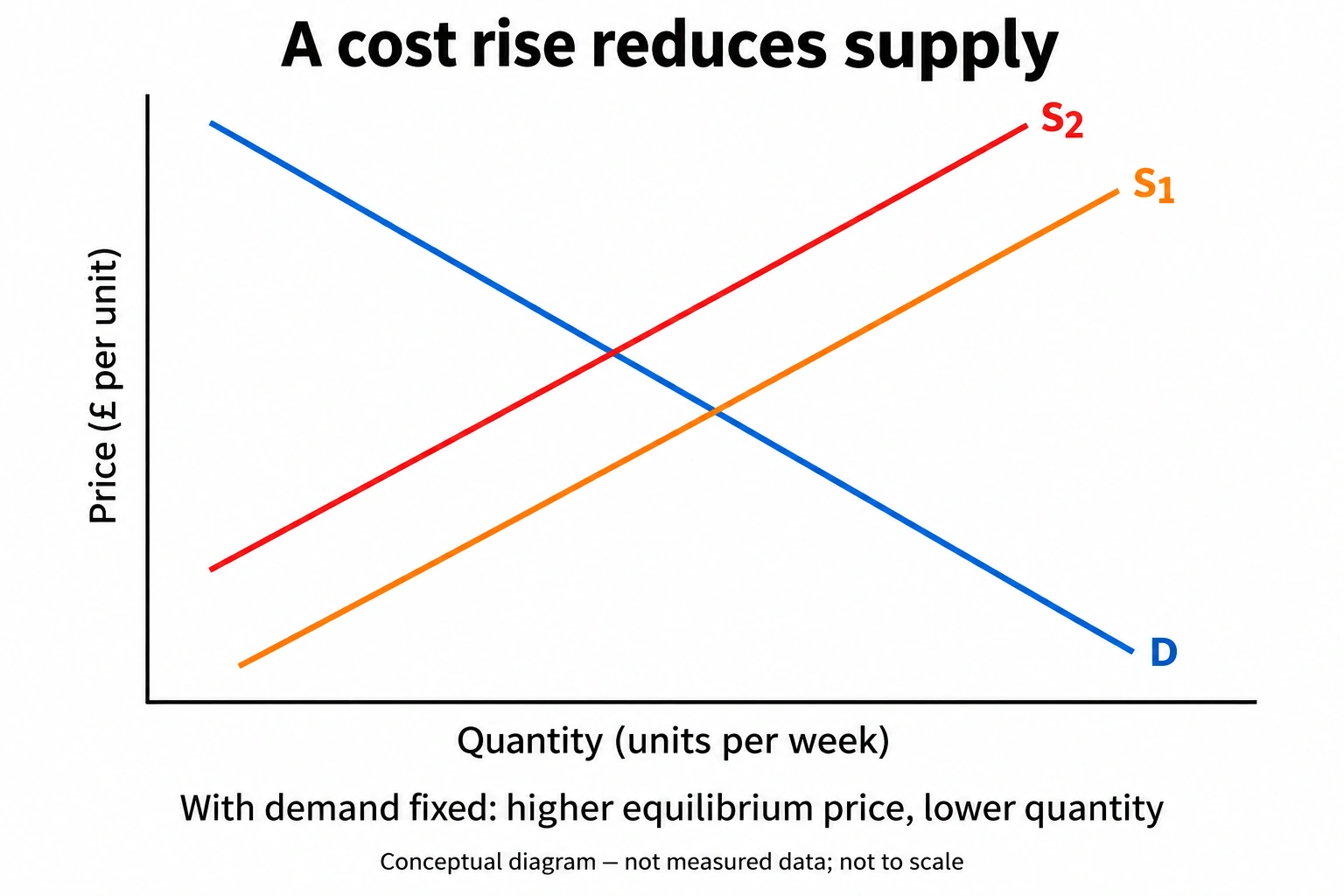
Original teaching plate generated using the built-in imagegen tool, 2026-10-04; conceptual or hypothetical, not empirical evidence. · Original generated artwork; provenance and rights acceptance pending independent review before public publication.
Supply: incentives, costs and the adjustment horizon
Supply is the quantity producers are willing and able to offer at alternative own prices over a period. The market supply curve usually slopes upward because higher prices can make additional output worthwhile. It is a conditional schedule, not a record of everything already sold. Quantity offered may exceed quantity purchased at a non-clearing price. Specify whether the unit is tickets, kilograms or hours and whether the period is a day or a year. A stock of stored goods measured on one date is not the same as units supplied each week, although releasing that stock can increase a weekly flow.
A higher own price, with other conditions fixed, causes a movement along supply. A change in input costs, productivity, technology, taxation, subsidies, producer numbers or expectations can shift supply. If electricity becomes dearer, producers may offer less at each output price, shifting supply up/left. A price rise caused by stronger demand can encourage more quantity supplied along the existing curve; that is not the same as a technological increase in supply. The plate shows a cost-driven leftward shift S1 to S2 with demand fixed. The higher intersection price and lower intersection quantity require demand interaction, not supply logic alone.
Time changes what can be adjusted. A bakery can extend shifts before it can build ovens, while a theatre cannot add seats tonight merely because tickets become expensive. Spare capacity, inventories, overtime and mobility can permit a fast response. Training, planning and capital investment take longer. Short run does not mean a universal number of months: it is a horizon in which at least one productive input is fixed. A positive supply response is plausible when expansion remains feasible and profitable; weather, biological growth and legal limits can prevent it even when incentives strengthen.
The usual competitive model treats sellers as too small to control the market price and able to respond to it. It also assumes a sufficiently well-defined product and workable access to information and exchange. A dominant seller may choose its price/output strategically, so a simple price-taking schedule can misdescribe its decisions. Supply is not defined by how generous firms are; even socially motivated producers face resource constraints. Likewise a cost reduction need not immediately lower a posted price if contracts or market power allow the firm to retain gains. Later market-structure lessons remain necessary before generalising competitive predictions.
Be precise about the causal direction. An observed rise in output and a rise in electricity use may reflect output causing input demand, not cheap electricity causing output. A report that both wages and supply rose could contain productivity growth offsetting labour-cost pressure. A diagram isolates one mechanism; evidence must identify which shifters actually changed. The worked equations below are invented schedules for learning, not an estimate of real firms' costs. They permit exact calculations while making the assumptions visible. Negative quantities outside the relevant range should not be interpreted as literal production.
When judging a subsidy or productivity intervention, connect the shift to implementation. A per-unit support payment can make more output worthwhile at a given buyer price, but funding has opportunity costs and verification may be difficult. A training grant may increase productivity only after trainees gain usable skills and remain in the industry. Firms may also respond by changing quality or recruiting from rivals, leaving total sector capacity unchanged. A strong conclusion states the horizon, the likely binding input and evidence needed about capacity and costs. Quantity supplied, sales, production and inventory changes are related but distinct flows.
Original model essay — part 1. Higher prices can encourage suppliers to offer more, but they cannot always eliminate a shortage quickly or without costs. Quantity supplied is an intended flow for a specified period, not the same as an existing stock or actual sales. A movement along a supply curve follows an own-price change with other influences held constant. A change in energy costs, technology or regulation changes the quantities offered at each price. Whether a price rise restores equilibrium therefore depends on the cause of the gap and on producers' feasible responses. The supply equations illustrate the distinction. Under the original schedule, Qs = 10P − 20, a six-pound price produces an offer of 40 units. A cost increase shifts the schedule to Qs = 10P − 40, reducing the offer at six pounds to 20. To offer 40 units under the new conditions requires a price of eight pounds. That is not the same event as a movement on the original schedule from six to eight, where offers rise from 40 to 60. None of these calculations identifies the market-clearing price without knowing demand. A theatre tonight has a particularly strong short-run capacity constraint. Higher prices may encourage the release of reserved seats or reduce the quantity demanded, but cannot instantly construct another auditorium. They may clear the market mainly by excluding customers with lower willingness or ability to pay. This can remove excess demand at the prevailing price while leaving unmet wants and distributional concerns. A price-clearing outcome is not evidence that everyone who would benefit from attending obtained a seat. Rules against overcrowding also mean some supposed supply responses are not feasible alternatives.
Original model essay — part 2. A bakery over a year has more scope to change output. It can adjust shifts, train staff or acquire equipment if expected revenue justifies the additional costs. Nevertheless, financing constraints, installation delays and uncertain future demand can limit the response. A temporary high price may not warrant a long-lived investment. The relevant comparison is the expected marginal revenue from extra sales against the marginal cost of supplying them, together with the risks and commitments that the model leaves implicit. A longer horizon often permits more adjustment, but does not guarantee unlimited elasticity. If energy costs rise while a production subsidy is introduced, the two changes can push supply in opposing directions. The cost rise tends to reduce offers at each price; a subsidy can increase the net return and encourage offers. Their magnitudes, eligibility rules and actual availability determine the net shift. Assuming that the subsidy entirely offsets the cost rise would be an unsupported numerical claim. Furthermore, a subsidy uses public funds with an opportunity cost, and may reward output that generates an external cost. The market quantity alone does not settle whether it improves welfare. I therefore reject the word always. Price adjustment can coordinate choices where offers and demand respond, but an immediate physical constraint may mean rationing mainly occurs through reduced demand. A durable solution may require capacity investment, better information or removal of a specific bottleneck. These alternatives also have costs. The appropriate policy depends on whether the problem is a temporary price-specific shortage, persistent limited capacity or a distributional objective that price clearing does not address.
Worked example: Hypothetical weekly output schedule Qs = 10P − 20, where P is £/unit and Qs units/week. A higher energy cost changes it to Qs = 10P − 40. Compare quantities at £6 and inverse prices for 40 units. Assume relevant non-negative range.
Initially at P=6: Qs=60−20=40 units/week. After the cost rise: Qs=60−40=20.
Initially Qs=40 requires 40=10P−20, so P=6. Afterwards 40=10P−40, so P=8.
The shift means 20 fewer units at each given price, or a £2 higher price required for a given quantity in this invented linear case.
At the original schedule, raising own price from £6 to £8 changes supplied quantity 40 to 60; this is a movement, not a shift.
No demand schedule has been supplied, so the calculated £8 is a supply offer price for 40 units, not a market equilibrium prediction.
Answer: At £6 supply falls 40→20 units/week. Supplying 40 requires £6 before and £8 after. The cost-driven shift must be distinguished from an own-price movement and from actual sales.
Check your understanding: Write 450–600 words assessing "Higher prices always solve a shortage by raising supply." Use a theatre tonight and a bakery over a year; include incentives, fixed inputs and an alternative explanation for persistent scarcity. Transfer: energy costs rise at the same time as a subsidy is introduced.
Answer: Higher prices can ration demand and encourage quantity supplied, but theatre seats tonight are fixed, so adjustment may occur mainly on the demand side. A bakery may add shifts quickly and ovens later, making its response larger over time. Staffing, planning and material constraints can remain. Higher energy costs shift supply left while a per-unit subsidy tends to shift it right; the net shift depends on their size and how they affect producers, not a rule that one always dominates. A price-controlled shortage can persist because posted prices cannot adjust, yet even a clearing market still faces scarcity. Best policy depends on the constraint, consumer access and costs of increasing capacity.
Why: Indicative criteria: supply definition with units/time; correct offer-price calculation; distinguish stocks from weekly flows and offered quantities from sales; analyse horizons using specific inputs; explain opposing cost/support mechanisms; judge the assertion conditionally with distribution and opportunity cost. A valid answer can favour price adjustment or capacity intervention if the binding constraints and policy costs are defended.