Simultaneous shifts and interrelated markets: what can be inferred?
By UK A Level Economics · independent study · myAudience
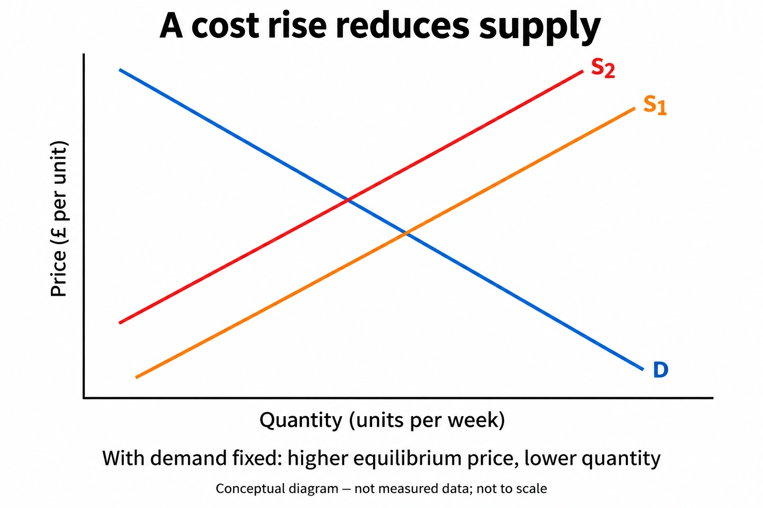
Original teaching plate generated using the built-in imagegen tool, 2026-10-04; conceptual or hypothetical, not empirical evidence. · Original generated artwork; provenance and rights acceptance pending independent review before public publication.
Simultaneous shifts and interrelated markets: what can be inferred?
One isolated shift yields a clear directional prediction under the usual curve slopes; two shifts may not. If demand rises while supply falls, both tend to raise price, but their effects on quantity oppose. Without relative magnitudes, quantity is ambiguous. If demand and supply both rise, quantity tends to rise while price is ambiguous. Ambiguous means the model and available evidence do not determine the sign, not that every outcome is equally likely. A careful economist states the determined result and identifies the missing information.
The supply plate fixes demand and therefore supports a higher-price/lower-quantity conclusion for a cost rise. It cannot by itself settle an event in which income also rises. To extend it, draw D2 right of D1 and compare the new intersection with the initial one. Do not place the final quantity merely where it looks convenient. A numerical specification can resolve the ambiguity; a qualitative scenario cannot do so without extra evidence. Moreover, the two supply curves are conceptual, so their pixel spacing cannot reveal how large a real cost shock is.
Markets transmit changes through economic relationships. Joint demand involves goods used together, such as printers and compatible cartridges. Competitive demand involves alternatives, such as bus travel and some bicycle journeys. Composite demand involves one input with several uses, such as timber for construction or furniture. Derived demand arises because an input is wanted for what it helps produce, such as labour for repairs. Joint supply occurs when one production process yields more than one output. These concepts describe mechanisms; naming a pair of goods is insufficient unless the relevant use or production connection is explained.
A rise in demand for repair services may raise demand for mechanics, increase wages and eventually draw workers from other occupations. That can affect other service prices. A crop used for food and fuel may become dearer when fuel demand rises, potentially reducing food use. Yet supply adaptation, import substitution or technological change may weaken the transmission. A partial-equilibrium diagram holds other markets fixed while analysing one. It is useful for isolating a first effect, but extended conclusions must consider feedbacks without treating every conceivable feedback as equally important.
Observed equilibrium outcomes do not identify which curve shifted. A price rise with unchanged quantity could result from demand expansion offset by supply contraction; it might also conceal quality changes, an administered price or aggregation across very different products. The worked example constructs two possible economies with the same demand increase and different supply losses. It shows why a conditional result is stronger than an unqualified prediction. The schedules are original hypothetical models; they should not be presented as measured evidence about an industry.
To evaluate a real explanation, organise evidence around discriminating predictions. Input-cost data support a supply mechanism; population, income or preference changes support demand; inventories and capacity inform timing. Evidence can still be endogenous: output expansion itself may bid up input prices. Choose a causal sequence, explain each link, and ask how a plausible alternative would affect your conclusion. A useful judgement might confidently predict dearer output while withholding a sales-volume prediction until magnitudes are known. This is not evasiveness; it is a precise boundary between what the model establishes and what requires measurement.
Original model essay — part 1. Dearer timber does not necessarily imply that less furniture will be sold. Timber is an input, so a higher input cost can reduce furniture supply at each furniture price. That mechanism raises the equilibrium furniture price and lowers quantity when furniture demand is unchanged. However, demand may change simultaneously, and the observed timber price can itself respond to furniture production. A useful explanation must distinguish the timber market, the furniture market and any related construction market instead of placing every change on one unnamed graph. The numerical examples show why quantity can be ambiguous. Starting with furniture demand Qd = 100 − 10P and supply Qs = 20 + 10P gives a price of four and quantity 60. If demand rises to 120 − 10P while supply falls to 10P, the new outcome is price six and quantity 60. A larger supply reduction, to 10P − 20, gives price seven and quantity 50. A smaller reduction, to 10 + 10P, gives price 5.5 and quantity 65. Prices rise in all three cases, but quantities remain constant, fall or rise. A housing boom could increase demand for timber through construction while also increasing demand for furniture to equip homes. Timber's higher price would then push up furniture costs, while stronger furniture demand offsets part or all of the quantity reduction. The net quantity outcome depends on the relative shifts and on the responsiveness of each schedule. Saying that the cost rise must dominate is an additional assumption, not a conclusion obtained from identifying an input relationship. Conversely, observing increased furniture sales would not prove that timber costs were irrelevant.
Original model essay — part 2. Derived demand adds reverse causation. If consumers independently become more willing to buy furniture, manufacturers may demand more timber to produce it. Higher timber prices can therefore be partly an effect of expanding furniture output rather than the original cause of reduced output. A study that treats the timber price as an entirely external shock risks confusing these directions. Information about when orders changed, which industries increased purchases and whether there was an independent timber supply disruption would help separate competing explanations. Related goods must also be classified for a specified use. Two materials can compete as inputs when producers substitute between them, while the same production process may require several complementary inputs. Joint supply is different: producing one output generates another output from the same activity. These relationships determine where a shock is transmitted. They should not be inferred merely because two prices move together, since a common change in energy costs or general demand can create co-movement without either good causing the other's price change. I would therefore conclude only that a timber cost increase, considered alone, puts downward pressure on furniture quantity. Predicting actual sales requires evidence on furniture demand and other supply conditions. The strongest investigation uses a clearly identified timber supply shock, examines substitutability and inventories, and compares firms with different timber exposure. Even that comparison needs assumptions about their customer markets. A conditional prediction is more informative than an absolute claim because it identifies the additional evidence capable of changing the conclusion.
Worked example: Use the initial Qd=100−10P, Qs=20+10P. Demand rises to 120−10P. In case A supply falls to 10P; in case B supply falls to 10P−20. Find each outcome and relate ambiguity to the original £4/60 equilibrium.
Case A: 120−10P=10P, so P=6 and Q=60 units/week.
Case B: 120−10P=10P−20, so 140=20P, P=7 and Q=50.
A smaller supply loss, to Qs=10+10P, would give P=5.5 and Q=65.
All three prices exceed £4, while final quantities can equal, fall below or exceed 60.
At relevant prices the schedules are non-negative. Different intercept shifts are illustrative assumptions, not inferred real measurements.
Answer: Case A £6/60; case B £7/50; smaller loss £5.50/65. Higher price is determined under these slopes; quantity requires relative shift magnitudes.
Check your understanding: Write 450–600 words assessing "Dearer timber must mean less furniture will be sold." Analyse construction demand, timber supply and furniture demand separately. Include a counterexample and a proposed evidence plan. Transfer: explain why greater furniture output could itself increase timber prices.
Answer: Construction demand can raise derived/composite demand for timber, making furniture inputs dearer and shifting furniture supply left. With fixed furniture demand that tends to reduce sales, but higher household income could raise furniture demand enough to offset it. The simultaneous-shift examples demonstrate unchanged, lower or higher quantity despite rising prices. Greater furniture production can itself increase derived demand for timber, creating reverse causation. Examine construction activity, timber harvest/import capacity, furniture incomes/preferences and timing; price/output correlation alone cannot settle the direction. A defensible conclusion treats the single-shock reduction as a conditional benchmark and judges likely magnitudes using evidence.
Why: Indicative criteria: distinguish timber and furniture markets; correctly apply derived/composite demand; identify determined and ambiguous results; give a valid numerical or diagrammatic counterexample; explain reverse causation and a discriminating evidence plan; make a bounded judgement. Do not require a guessed quantity direction when the scenario does not supply magnitudes. Reward economic coherence over the number of technical labels.