Price allocation and surplus: private gains versus social welfare
By UK A Level Economics · independent study · myAudience
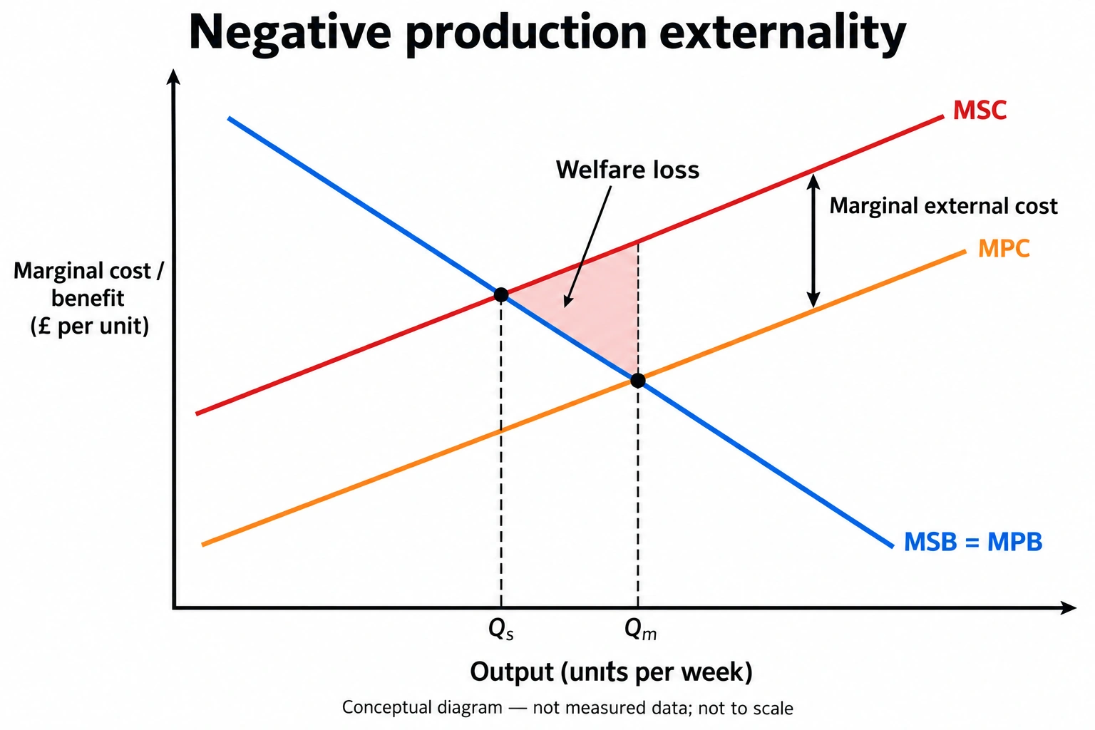
Original teaching plate generated using the built-in imagegen tool, 2026-10-04; conceptual or hypothetical, not empirical evidence. · Original generated artwork; provenance and rights acceptance pending independent review before public publication.
Price allocation and surplus: private gains versus social welfare
Prices ration limited output, signal scarcity and create incentives to alter use and production. A higher price can discourage low willingness-to-pay purchases and encourage supply expansion, coordinating decisions without a central list of every preference. These functions explain a mechanism, not an ethical verdict. Ability to pay affects demand, so high need can coexist with low effective demand. Introducing prices into a new activity may also change motives or trust. Evaluate what information the price communicates, which costs it omits, and who is excluded before treating allocation by willingness to pay as socially best.
Consumer surplus is the gap between willingness to pay and the price paid, summed over traded units. Producer surplus is receipts above the minimum amounts needed to supply those units, represented above the supply curve and below price in a competitive diagram. Producer surplus is not identical to profit: fixed costs can remain to be deducted. With linear curves and a uniform clearing price, each area is a triangle. Multiplying a price difference in £/unit by a quantity in units/week gives £/week. State those units to avoid treating a diagram area as an unexplained number.
For a no-externality competitive benchmark with reliable information, marginal willingness to pay can represent marginal private benefit and supply can represent marginal private cost. Total private surplus is maximised where those marginal values match; extra units beyond that point cost more than buyers value them, while units before it can yield additional net gains. This result requires assumptions about external effects, information and the welfare criterion. It is not a theorem that an unequal distribution is fair. Willingness to pay depends on income, and a pound may have different welfare significance to different people.
The externality plate introduces the reason private surplus can mislead. MPC omits marginal external harm, while MSC includes it; the privately traded Qm exceeds the social benchmark Qs. We will calculate that divergence in lesson 13. Here use the plate to notice that the extra private transactions between Qs and Qm need not raise social welfare. Do not measure the shaded area from pixels: it is conceptual. Nor is every high price an externality. Monopoly restrictions, information problems and distributional concerns involve different mechanisms and need their own models.
Allocative efficiency in a standard marginal model uses equality of marginal social benefit and marginal social cost. Productive efficiency concerns producing an output at the least relevant resource cost; dynamic efficiency concerns improvement through innovation and investment over time. A static low-price outcome might coexist with inadequate innovation, or investment might improve future quality while raising current costs. This first lesson establishes the distinctions but does not teach the full firm diagrams or close market-structure requirements. An extended evaluation should identify which efficiency concept a claim invokes rather than moving unnoticed between them.
A subsidy, tax or restriction redistributes gains as well as changing traded quantity. Government receipts are not automatically a welfare loss, and payments to producers are not automatically a benefit net of their funding. A rigorous response tracks consumers, producers, government and affected third parties, then checks for double counting. It also states whether the judgement treats each pound equally or gives distributional weight to disadvantaged groups. Those normative choices can be defended, but they should be visible. Quantitative surplus is a disciplined benchmark, not a substitute for all dimensions of welfare.
Original model essay — part 1. Maximising consumer and producer surplus is a useful competitive benchmark, but it is not sufficient by itself to identify the best policy. Consumer surplus measures willingness to pay above expenditure, while producer surplus measures receipts above the relevant variable supply costs. Neither measure automatically includes all external effects, distributional priorities or future benefits. Producer surplus is also not identical to profit when fixed costs remain. A policy judgement must state which welfare criterion is being applied and why the model's boundaries are appropriate. In the hypothetical inverse schedules, demand is P = 10 − 0.1Q and supply is P = 2 + 0.1Q. Equating them gives Q = 40 and P = 6. Each triangular surplus is one half multiplied by 40 and four, or 80, so their sum is 160. With a two-pound per-unit tax, buyer price becomes seven, seller net price five and quantity 30. Consumer and producer surpluses fall to 45 each, while tax revenue is 60. Counting only the private surpluses would exaggerate the aggregate loss by ignoring revenue as a transfer within the stated accounting boundary. The combined total after tax is 150, giving a ten-unit deadweight loss under the no-externality assumptions. Its interpretation is the lost gains from the transactions between quantities 30 and 40, not every pound paid in tax. Whether the government spends revenue efficiently is a further question. It would be equally mistaken to count the revenue once as an included transfer and then count its full value again as an additional benefit without specifying the public-service costs and benefits. A transparent boundary prevents attractive-looking but inconsistent welfare totals.
Original model essay — part 2. An externality changes the benchmark. If production imposes costs on others that are absent from the supply schedule, private surplus maximisation can produce too much output. The externality plate explicitly distinguishes marginal private from marginal social cost. A tax that reduces private surplus may improve social welfare by avoiding damage, provided it targets the relevant margin and its implementation costs do not outweigh the gain. The original ten-unit calculation cannot then be reused as the full social loss without adding the omitted external-cost relationship. Distribution matters independently. Willingness to pay reflects ability to pay, so a gain to wealthy purchasers may dominate the monetary total even when a different allocation meets a social access objective. Weighting gains differently is a normative decision that should be made explicit. Producer surplus may also finance investment, but treating all retained surplus as productive investment would require evidence. A policy that reduces current surplus could improve future productivity through education or infrastructure, yet expected benefits should account for uncertainty, delay and the resources used. A promised future gain is not the same as an achieved gain. I would use the surplus model as a disciplined starting point: identify transfers, genuine resource costs and marginal external effects. I would then examine distribution, dynamic consequences and feasible policy alternatives. Under competitive conditions with no omitted effects and an accepted monetary welfare criterion, surplus maximisation can be a persuasive recommendation. Where those assumptions fail, insisting that the largest private-surplus sum defines the best policy silently answers ethical and empirical questions that the diagram cannot settle. The strongest conclusion is conditional and explains which additional evidence or value judgement would change it.
Worked example: Hypothetical inverse demand P=10−0.1Q and inverse supply P=2+0.1Q, Q units/week. Find equilibrium and linear consumer/producer surplus. Then impose the £2/unit tax. Assume no externalities, no admin cost and unchanged schedules.
Before tax 10−0.1Q=2+0.1Q gives Q=40 and P=6. Consumer surplus = 0.5×(10−6)×40=£80/week.
Producer surplus = 0.5×(6−2)×40=£80/week. Total private surplus = £160/week; fixed costs are not specified.
With tax, buyer price minus seller price=2: (10−0.1Q)−(2+0.1Q)=2 gives Q=30, Pc=7 and Ps=5.
Consumer surplus=0.5×3×30=£45; producer surplus=£45; tax revenue=2×30=£60. Combined = £150/week.
Loss = £10/week, equivalently 0.5×tax wedge £2/unit×quantity reduction 10 units/week. The £60 transfer is included, not counted as lost.
Answer: Before tax £80 consumer and £80 producer surplus. After: £45 each plus £60 receipts, leaving a £10 weekly benchmark loss. This result depends on no external harm; fixed costs and distribution are separate.
Check your understanding: Write 500–650 words evaluating "Maximising consumer and producer surplus is sufficient to decide the best policy." Use the tax example and externality plate. Consider low-income consumers and a future productivity gain; make a justified final judgement.
Answer: The surplus calculation provides a transparent static benchmark and prevents treating all tax revenue as lost. Without externalities/admin costs, the £2 tax reduces combined surplus by £10/week. With external harm, reduced output may improve social welfare because private supply omits costs; the same tax cannot be judged from private areas alone. Income affects willingness to pay, so unweighted monetary surplus need not settle distributive fairness. A future productivity improvement can add dynamic benefits requiring a time horizon and uncertainty assessment. Use surplus as one input, then include third parties, distribution, future effects and implementation. A conclusion favouring a tax or rejecting it needs those conditions, not an automatic preference for either markets or intervention.
Why: Indicative criteria: correct triangles and units; distinguish producer surplus from profit; include receipts without double counting; explicitly identify welfare assumptions; connect distribution and future productivity to the criterion; give a reasoned judgement. Reward a different normative weighting if openly justified. Full monopoly and innovation models remain outstanding, so do not claim this exercise proves a complete efficiency ranking.