Inflation, unemployment and the macro dashboard: reading rates carefully

By UK A Level Economics · independent study · myAudience

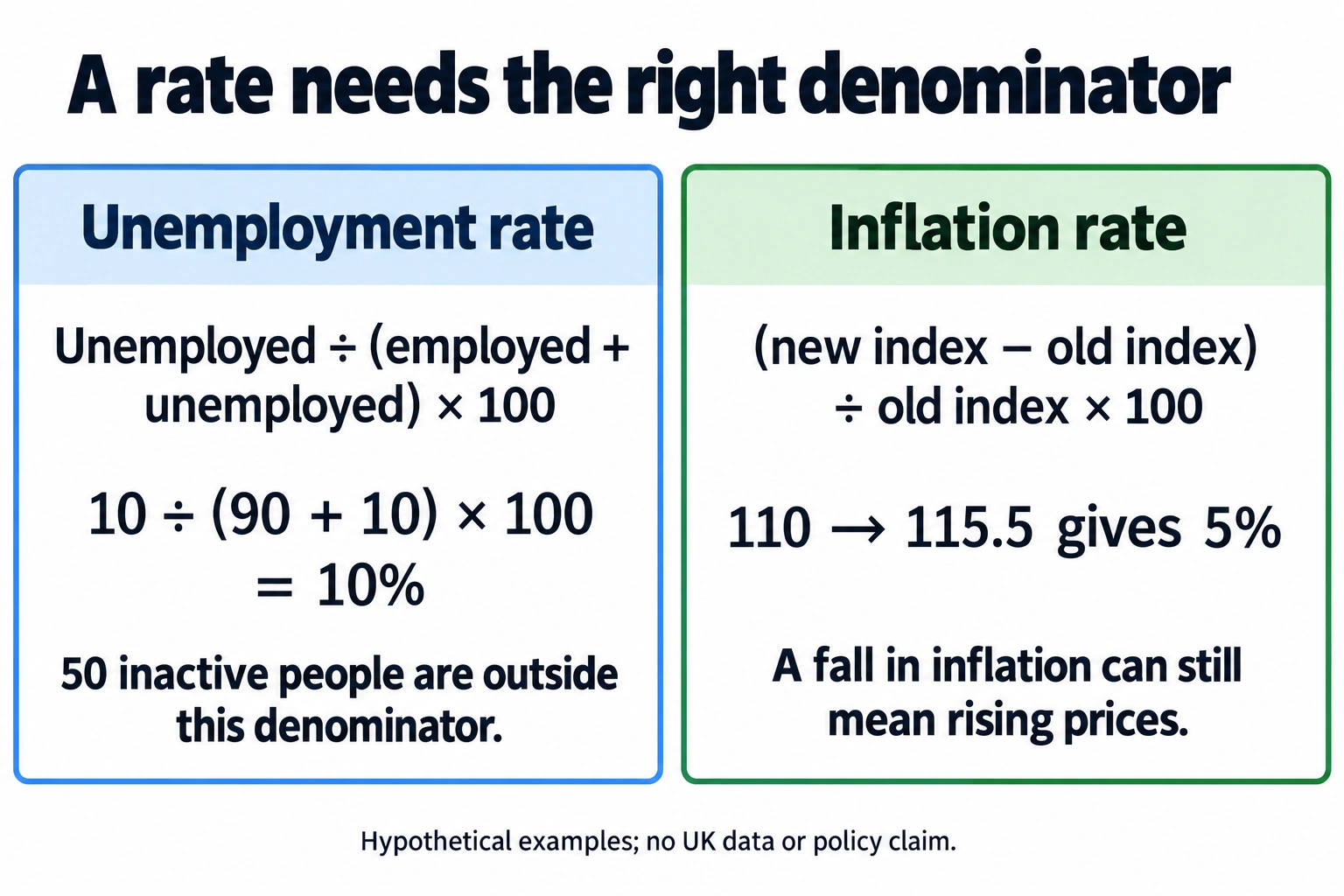
Original teaching plate generated using the built-in imagegen tool, 2026-10-04; conceptual or hypothetical, not empirical evidence. · Original generated artwork; provenance and rights acceptance pending independent review before public publication.

Inflation, unemployment and the macro dashboard: reading rates carefully

A price index expresses prices relative to a base period, commonly set to 100. Inflation is a rate of change in a general price level over a stated interval, not the level of the index itself. An index of 115.5 does not mean inflation is 115.5%. If it was 110 a year earlier, annual inflation is 5%. Disinflation means inflation falls; prices can still rise. Deflation means the price level falls. A single expensive item does not by itself establish general inflation, and a falling price in one category can coexist with a rising weighted basket.

A simple classroom weighted price index combines price relatives with expenditure-share weights summing to one. If food has weight 0.4 and its relative price is 120, while other goods have weight 0.6 and relative price 105, the index is 111. This is an illustrative fixed-basket calculation, not the complete ONS method. ONS aggregates detailed prices and updates weights; a national index is not each household's personal cost-of-living change. Different expenditure patterns, substitutions and quality changes matter. CPI and RPI have different coverage and methods and should not be assumed interchangeable; the specification requires awareness, not detailed technical reconstruction.

Unemployment is not everyone without a job. The ONS internationally based definition includes people without work who actively sought it in the previous four weeks and can start in the next two, plus those waiting to start a job already obtained within two weeks. People outside those conditions may be economically inactive. The unemployment rate divides unemployed people by the labour force—employed plus unemployed—not the total population. The plate makes the denominator explicit. The claimant count uses benefit-related administrative conditions and need not match the survey measure; current eligibility or numerical rates require dated evidence.

A falling unemployment rate can accompany fewer jobs if people leave the labour force. Similarly, employment can rise while productivity per worker falls if hours or output change. Labour productivity is output per worker or per hour, depending on the stated denominator, not total output. Seasonal patterns, survey error, revisions and changing participation complicate comparisons. Use matched periods and populations. Do not infer that a lower unemployment rate proves a successful policy without a counterfactual; demand conditions, ageing, education participation or migration can provide competing explanations.

Government objectives commonly include output growth, price stability, low unemployment and a sustainable external position. Their priority and potential conflicts need analysis, not a claim that one number should always dominate. A current-account balance is a flow over a period, containing goods, services, primary income and secondary income; it is not the total wealth owed abroad. A deficit does not alone prove poor performance, and a surplus does not automatically prove success. Explaining their causes and financing requires later international lessons. Here build a measurement dashboard and distinguish an indicator from an explanation or value judgement.

Join indicators rather than treating them as a league table. Nominal output rising while inflation rises may conceal little real expansion; output per head can move differently from total output. Falling unemployment with shrinking labour-force participation suggests a different story from rising employment. An index change may affect lower-income households differently because spending shares differ. A good extended response calculates, checks units and denominators, offers at least two plausible mechanisms and states additional evidence needed. The examples are hypothetical, not current UK data; no policy success or failure is claimed from them.

Original model essay — part 1. Lower unemployment and lower inflation do not establish that everyone is better off. Both indicators have precise denominators and definitions, while welfare concerns individuals with different employment, income and spending circumstances. Falling inflation means slower price growth, not necessarily falling prices. A lower unemployment rate can reflect people finding work, but it can also arise when people stop meeting the unemployment definition and leave the labour force. The appropriate judgement examines the mechanisms behind the rates and their distribution, rather than treating a favourable direction as a complete outcome. The labour-force example begins with 90 employed people, ten unemployed and 50 inactive. The unemployment rate is ten divided by 100, or 10%; inactive people are excluded from that denominator. Later, employment is 88, unemployment eight and inactivity 54. The unemployment rate becomes eight divided by 96, approximately 8.33%. It falls by about 1.67 percentage points even though employment falls by two people, approximately 2.22%. Participation drops from 100 out of 150, about 66.67%, to 96 out of 150, or 64%. These changes demonstrate why the headline rate cannot by itself establish labour-market recovery. Evidence on movements between employment, unemployment and inactivity would help distinguish discouraged jobseekers from voluntary retirement, education or caring decisions. The survey definition includes specified search and availability conditions, with an additional route for people waiting to start a job; it is not simply the number receiving a particular benefit. Job quality, hours, earnings and accessibility also matter. More employment could be beneficial while involving insecure or low-paid work, and fewer working hours could be voluntary or involuntary. Judgement therefore needs specific evidence about the people affected, not a presumption that every movement out of unemployment is the same.

Original model essay — part 2. Inflation requires similarly careful interpretation. An index rising from 100 to 110 and then to 115.5 implies inflation falling from 10% to 5%, while prices continue to rise. In the separate weighted-basket example, 40% food at index 120 and 60% other goods at 105 gives an index of 111. Relative to a matched prior index of 105, the increase is six divided by 105, approximately 5.71%. A household spending 70% on food and 30% on other goods has a current weighted index of 115.5. Its inflation rate still requires its own matched prior basket; assigning the aggregate prior index of 105 without justification would fabricate a comparison. The productivity transfer adds another distinction. If real GDP rises but total hours worked rise faster, real output per hour falls. Higher production alone therefore does not establish improved productivity, just as a lower unemployment rate does not establish more jobs. Evidence on hours, capital use and output quality would be needed to explain the change. The consequences for individuals depend on earnings and working conditions; an output gain achieved through much longer unwanted hours could have a different welfare significance from the same gain produced more efficiently. My judgement is that lower rates are useful signals requiring decomposition, not proof of universal improvement. I would combine employment and participation, real earnings and hours, matched price measures and distributional evidence. Some households may benefit from slower price growth while others still lose purchasing power or leave work involuntarily. The supplied figures explicitly show potentially favourable headline movements alongside adverse underlying changes. A persuasive conclusion states which groups gain, which mechanism caused the movement and what counterfactual supports calling it an improvement.

Worked example: Hypothetical basket weights food 0.4 and other goods 0.6; current relative prices 120 and 105 (base=100). Prior-year index 105. Labour market before: 90 employed, 10 unemployed, 50 inactive; after: 88 employed, 8 unemployed, 54 inactive, same total 150.

Weighted index=0.4×120+0.6×105=48+63=111. Against prior 105, inflation=(111−105)/105×100≈5.714%.

Before unemployment rate=10/(90+10)×100=10%; after=8/(88+8)×100≈8.333%. The decline is about 1.667 percentage points.

Employment nevertheless falls by 2, or 2/90×100≈2.222%. Participation falls from 100/150≈66.667% to 96/150=64%.

A household weighting food 0.7 and other goods 0.3 would have a simplified current index 0.7×120+0.3×105=115.5. Its inflation needs its own prior index, not automatically the national 105.

If an index rises 100→110→115.5 in successive years, inflation falls 10%→5% while the price level continues to rise.

Answer: National illustrative index 111 and annual inflation about 5.714%. Unemployment falls 10%→8.333% despite lower employment and participation. Disinflation need not mean falling prices; personal index inflation needs a matched personal base.

Check your understanding: Write 500–650 words evaluating "Lower unemployment and lower inflation prove every household is better off." Use the numbers and plate, distinguish percentage changes from percentage points, and propose evidence to separate recovery from labour-force exit. Transfer: real GDP rises but hours worked rise faster.

Answer: The unemployment-rate decline is 1.667 percentage points, while employment falls about 2.222% and participation falls. Labour-force exit can reduce the rate without new jobs, so examine flows, hours and inactivity reasons. Disinflation leaves prices rising; real wages and household-specific baskets determine purchasing-power effects. An aggregate index does not measure each household's experience. If real GDP rises more slowly than hours, output per hour falls despite higher total production. Add real median incomes, employment/hours/participation and distributional price evidence with matched periods. A bounded judgement recognises potentially favourable indicators but rejects proof of universal gains or a causal policy effect.

Why: Indicative criteria: correct weighted index and prior-year inflation denominator; correct labour-force denominator, employment/participation rates and percentage-point distinction; define disinflation/deflation; handle household weights without inventing a prior index; distinguish productivity from production; propose a causal evidence plan and a justified judgement. Reward another plausible mechanism if consistent with the arithmetic and explicitly conditional.