Describing data without hiding their structure

By UK A Level Psychology · independent study · myAudience

myAudience original rendered educational illustration. Image: illustration, not a documentary photograph. · Generated for this isolated pending curriculum pack; no third-party artwork licence claimed.

Describing data without hiding their structure

Before choosing a statistic, ask what each number represents and which observations belong together. Nominal measurement classifies without a numerical order, such as agree/disagree categories. Ordinal measurement orders values without established equal intervals, such as ranked confidence. Interval measurement assumes equal differences have comparable meaning; an arbitrary attitude rating is not made interval merely by printing digits. A count of correctly recalled words has equal count increments, but the psychological distance between successive scores need not be identical. uses nominal, ordinal and interval in test selection; more detailed measurement debates remain relevant when judging assumptions.

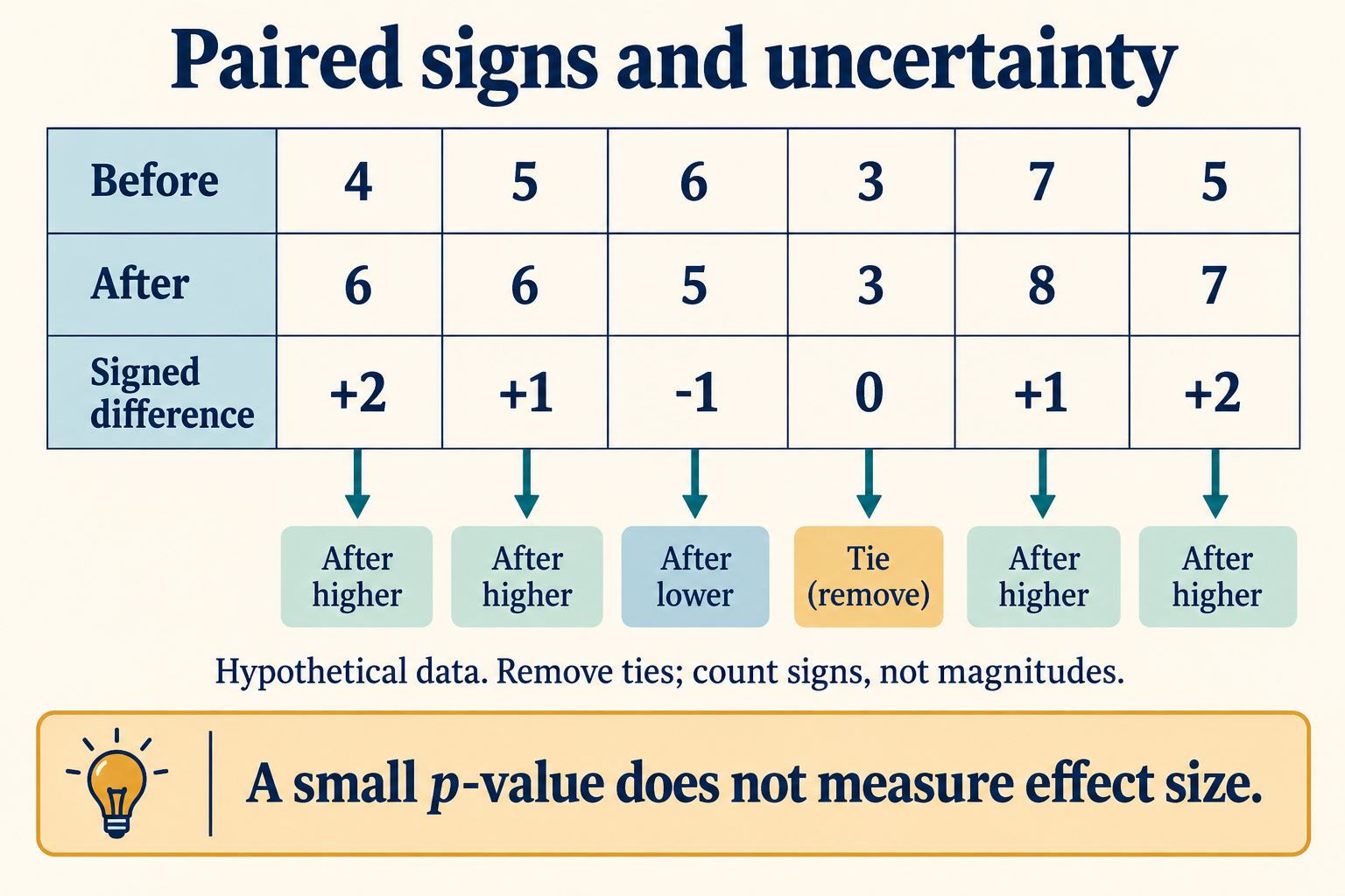
The mean uses every value and preserves arithmetic information but can be pulled by an extreme score. The median identifies the middle of the ordered values and resists a single extreme better. The mode is the most frequent value and can describe a nominal category; a dataset can have several modes or no unique one. Select a summary in relation to the distribution and question rather than declaring a measure universally best. For paired data, the mean difference is usually more informative about change than two unrelated summaries, while a table of individual differences shows whether a mean advantage is broadly shared or driven by one participant.

Range is maximum minus minimum, so it uses only two scores. Standard deviation describes spread around the mean using every score. For the sample convention used here, subtract the sample mean from each score, square the deviations, add them, divide by n−1, and take the square root. The result has the original outcome's units; variance has squared units. If an exam supplies a formula with divisor n, follow that formula and explain the convention rather than silently switching denominators. The revised specification's mathematics annex explicitly includes calculating standard deviation, so naming it without performing and interpreting a calculation leaves a gap.

A roughly normal distribution is symmetric and bell shaped, with mean, median and mode together in the ideal case. In a positively skewed distribution a long upper tail usually pulls the mean above the median; negative skew reverses the usual direction. These are characteristic patterns, not guarantees for every tiny dataset. A ceiling in a twelve-word test piles scores near twelve and can conceal differences between strong performers. Lowering task difficulty may make that worse, while lengthening a list changes the task itself. Report the distribution and measurement ceiling instead of interpreting a small condition difference as a universal absence of memory differences.

Tables preserve exact values and pairing. Bar charts compare distinct categories; bars are separated because the categories are not adjoining numerical intervals. Histograms describe distributions across continuous numerical intervals, with adjacent bars; unequal-width intervals require attention to frequency density rather than misleading raw heights. A scattergram puts each person's two measurements together as one point. A positive correlation means larger values of one tend to accompany larger values of the other; a negative correlation means the opposite. A coefficient near zero indicates little linear or monotonic association of the relevant kind, not necessarily no possible relationship. A U-shaped pattern can evade a single linear summary.

The paired-signs image intentionally discards magnitudes in its sign labels. Its four increases, one decrease and one tie are different information from its mean change of one word. The picture is hypothetical and supplies no population estimate. An extended model can separate average change, variability and the proportion changing in the expected direction. All three could matter: a small mean could hide large opposite individual changes, and a consistent small change could matter differently from a variable large change. Keep precision honest by retaining working values then rounding final results appropriately; 4.6904 words becomes 4.69, not evidence that recall was measured to hundredths of a word.

Worked example: Hypothetical recall scores are 2,4,4,6,14 words on a longer-than-fourteen-word task. Find mean, median, mode, range and sample SD. Compare with the first four scores alone. Explain why removing the fifth score merely to get a tidier result is unacceptable.

With all five scores, total=30 and mean=6. Ordered median=4, unique mode=4 and range=14−2=12 words.

Deviations from 6 are −4,−2,−2,0,8. Squared deviations total 88; sample variance=88/(5−1)=22; SD=√22≈4.69 words.

Without 14, mean=4, median=4, mode=4 and range=4. Squared deviations total 8; sample SD=√(8/3)≈1.63 words.

An extreme observation is not automatically an error. Check a predefined eligibility or scoring rule, disclose any legitimate correction, and show sensitivity to retaining the score.

Answer: The fifth score raises the mean and spread but leaves the median and mode unchanged. Median 4 is a useful typical-score summary here; the full table and justified inclusion rules preserve evidence of variation.

Check your understanding: Transfer: a histogram uses bands 0–4 and 4–12 with frequencies 8 and 8. A researcher gives both bars equal height and says the distribution is uniform. Explain the problem. Also interpret a scattergram with high scores at both very low and very high values of a co-variable.

Answer: The intervals have widths 4 and 8, so equal frequencies imply densities 2 and 1 per unit, not equal density. Equal raw bar heights misrepresent an unequal-width histogram. The scattergram suggests a possible non-linear U-shaped association; a near-zero Pearson coefficient would not exclude it. Inspect plots before summarising.

Why: Indicative rubric: credit a correct SD convention and units, resistance to arbitrary outlier removal, frequency density and the non-linear alternative. Do not award a causal interpretation of correlation or a claim that an exact small-sample histogram must follow a normal distribution.