6. Hydrographs: peaks, lags and conserved storm volume

By UK A Level Geography · independent study · myAudience

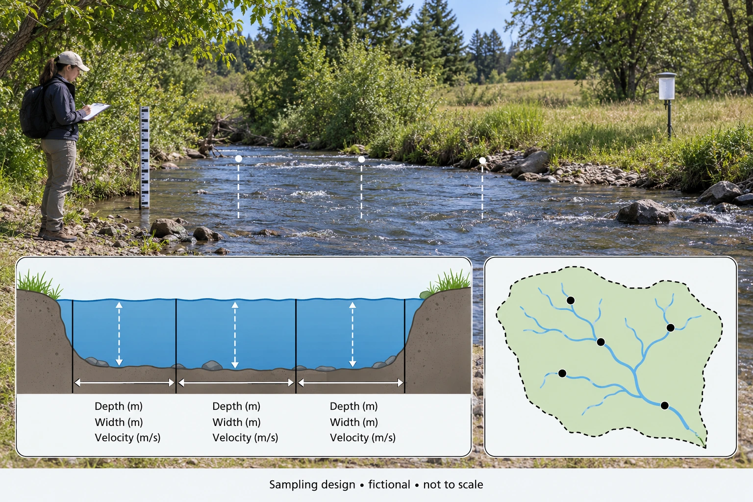
Image: illustration, not a documentary photograph. · Original generated teaching artwork; provenance retained. No, government or research-body endorsement.

6. Hydrographs: peaks, lags and conserved storm volume

A flood hydrograph plots river discharge against time. Discharge is a volume rate in m³/s, not a water level or rainfall depth. The rising limb indicates increasing outlet flow; the recession records declining flow. Peak discharge matters for channel capacity, while the volume under the curve matters for the event budget. Lag must have a stated convention, such as rainfall-intensity peak to discharge peak or rainfall centroid to runoff centroid. Different conventions can produce different values. A single plotted lag is therefore not comparable across studies unless the definitions match.

Baseflow is slower release, often supplied by groundwater, that continues between storms. Direct runoff separation subtracts an estimated background from total discharge. The background may itself change during a storm, so a constant subtraction is a simplified model. Integrating samples with the trapezoidal rule assumes a straight-line segment between observations. Sparse readings can miss the true peak, and a recession truncated at the final sample excludes later water. A calculation can be correct for the supplied curve while understating actual event volume.

Converting runoff volume to basin depth allows comparison with rainfall. Divide volume by basin area in square metres and multiply metres by 1,000 for millimetres. A storm runoff coefficient is direct-runoff depth divided by storm rainfall depth. It need not describe the annual balance, and it depends on event definition and separation assumptions. A coefficient greater than one could reveal release of pre-existing water, imported water, rainfall undercatch or misaligned intervals. It should prompt investigation, not automatic deletion of the inconvenient result.

Sharper hydrographs may reflect connected impervious surfaces, steep slopes, low storage capacity or wetter initial conditions. Geology and channel routing can sustain a gentler response. To infer the influence of development, compare similar rainfall patterns and antecedent states or use a model whose predictions are independently tested. Even if an intervention reduces the local peak, it may shift timing so that downstream tributaries peak together. Basin-scale risk requires routing and confluence information, not just one monitoring station's maximum.

The measurement plate places depth and velocity observations within a channel section. It does not contain a numerical hydrograph; learners must construct that from the tabulated data. Put time on the horizontal axis and discharge on the vertical axis with units, plotting total discharge and the assumed baseflow separately. Do not make the curve smooth merely for appearance if that implies unobserved features. Indicate the sample points and interpolation assumption. This makes the difference between source readings and modelled between-sample values visible.

When arguing whether 'slowing the flow' works, specify the target: lower peak, lower volume, longer warning time, less damage or greater resilience. These are related but not interchangeable. Storage can redistribute a fixed runoff volume over time without changing it, whereas infiltration or evaporation can reduce the amount reaching the channel in the event window. A justified conclusion recognises both mechanisms and the monitoring limits. All values in the application are original fictional readings, not a real station record.

Worked example: Fictional basin area 2 km², storm rainfall 30 mm. At t = 0, 1, 2, 3, 4 hours, total Q = 2, 8, 14, 8, 2 m³/s. Assume constant baseflow 2 m³/s and zero event excess after hour 4. Rain intensity peaks at hour 0.5. Calculate direct volume, depth, coefficient and peak-to-peak lag. A storage option changes total Q to 2, 6, 10, 10, 6, 2 at hours 0–5: compare peak and volume.

Evaluated extension (original task): Evaluate whether a lower peak proves both less runoff and less flood damage.

Subtract baseflow: original excess is 0, 6, 12, 6, 0 m³/s. Trapezoid areas total 24 (m³/s)·hours; multiply by 3,600 to get 86,400 m³.

Depth = 86,400 / 2,000,000 × 1,000 = 43.2 mm; coefficient = 43.2 / 30 = 1.44.

Peak-to-peak lag = 2 − 0.5 = 1.5 hours. A coefficient above one means the simple event assumptions need checking; it is not proof of water creation.

Option excess 0, 4, 8, 8, 4, 0 integrates to the same 24 rate-hours. Total peak falls from 14 to 10 m³/s (28.6%), while direct volume remains 86,400 m³.

A lower peak is not synonymous with less runoff or less damage. Subtracting the 2 m³/s baseflow and integrating the original hourly series as piecewise-linear segments gives 86,400 m³ of direct flow. The alternative five-hour series gives the same volume, although its total-flow peak is 10 m³/s rather than 14 m³/s. The reduction in the observed total-flow peak is 28.57%. This can matter for a local capacity threshold, but it does not establish that water has disappeared from the catchment. The model illustrates retiming of release, and the longer event must be included when comparing the two volumes.

The event water check also limits interpretation. A 30 mm rainfall total over 2 km² supplies 60,000 m³, whereas the direct-flow estimate is 86,400 m³, equivalent to 43.2 mm. Its coefficient is 1.44. That does not authorize water creation; under the chosen account, at least 26,400 m³ must come from prior storage or another input, unless the observations or boundary are wrong. Calling flow above a simple baseline 'direct' does not prove that every litre is newly fallen rain. A defensible explanation distinguishes baseflow subtraction, event water origins and measurement uncertainty rather than silently forcing the coefficient below one.

Flood damage depends on more than a single peak at one gauge. A later release may coincide with another tributary downstream, or a prolonged moderate flow may still exceed a critical local level. Damage also depends on exposure, building vulnerability, warning and protection. The conceptual retention plate cannot establish a measured delay or capacity: storage is finite and outlets continue releasing water. Comparison requires consistent sampling intervals and interpolation, because sparse readings can miss a short-lived peak. The assumed constant baseflow is another simplification; if actual background flow varies, direct-volume estimates and the inferred coefficient would change.

I would conclude that the supplied alternative preserves runoff volume while reducing and extending the local total-flow peak. I would only infer a damage benefit where relevant thresholds, downstream timing and exposed assets support it. A stronger evaluation would use matched events, upstream and downstream observations, independent rainfall measurements and uncertainty around the intervention counterfactual. If a delayed peak moves safely below a vulnerable location's threshold without worsening another location, the case is persuasive. If releases coincide downstream or storage fills earlier than assumed, it weakens. Peak, volume, timing and consequences are therefore linked evidence, but none can substitute for the others.

Answer: The option lowers the sampled peak but conserves the supplied direct volume. The rainfall input is only 60,000 m³, so the original event has a 26,400 m³ excess over rainfall; release of initial storage or errors/omissions must explain it.

Check your understanding: Transfer: suppose independent groundwater evidence supports release of 13.2 mm of initial stored water, with negligible ET during this event. Is the coefficient then physically possible? What remains unproven about the option?

Answer: Yes: 30 mm rain plus a 13.2 mm store loss can supply 43.2 mm runoff. The coefficient is a ratio to new rainfall, not a requirement that no old water leaves. The option still lacks proof of downstream timing, overflow performance and actual damage reduction; its sampled curve is a fictional counterfactual.

Why: The apparently anomalous coefficient is intentional. A conservation check forces a causal interpretation and exposes the limits of equating a lower peak with less water.