7. Discharge measurement: uncertainty, bias and spatial sampling

By UK A Level Geography · independent study · myAudience

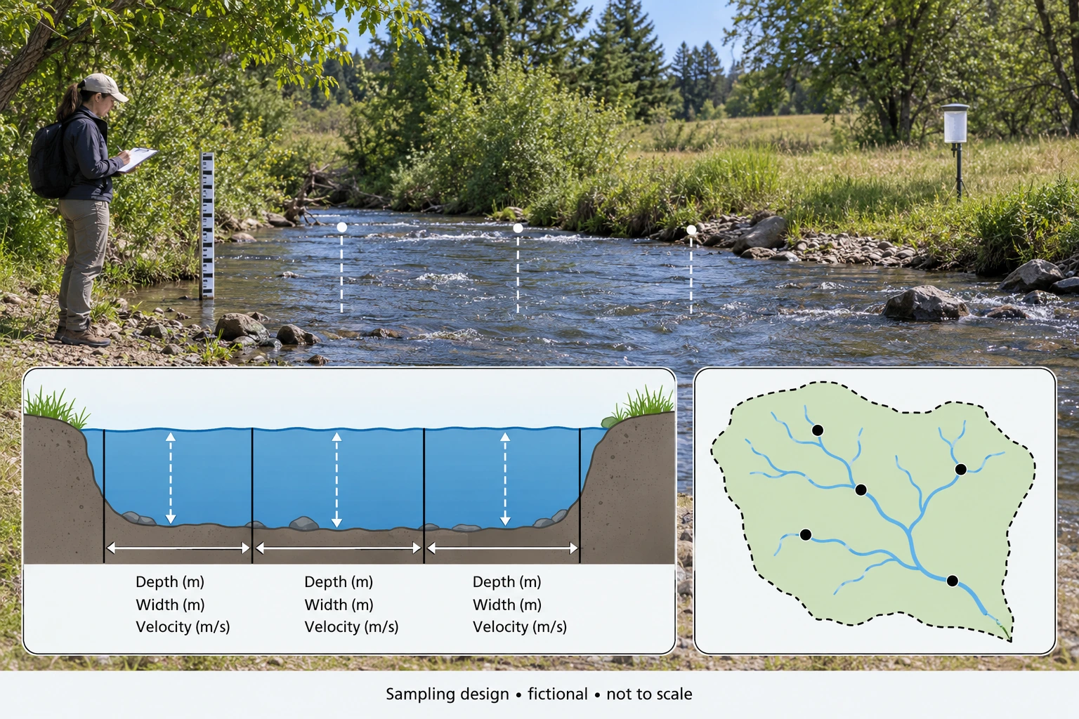
Image: illustration, not a documentary photograph. · Original generated teaching artwork; provenance retained. No, government or research-body endorsement.

7. Discharge measurement: uncertainty, bias and spatial sampling

Field data do not become reliable merely because they are numerical. Repeatability describes consistency under similar conditions; accuracy concerns closeness to the quantity sought; representativeness concerns whether the sample covers the relevant space, time and population. A velocity instrument can repeat a biased reading very precisely. Measurements taken only beside an accessible bank may systematically miss the faster channel centre. Rain gauges clustered near roads may miss an upland rainfall gradient. These errors have different remedies: replication helps random variation, calibration helps instrument bias, and sampling design helps coverage.

A velocity–area estimate divides a stream cross section into strips, estimates each strip's wetted area and representative mean velocity, then sums area × velocity. Width in metres times depth in metres gives m²; multiplying by m/s gives m³/s. In natural channels strips are not generally perfect rectangles, and velocity changes vertically and laterally. A surface float often travels faster than the depth-mean flow; applying a coefficient without local validation introduces model uncertainty. The method is an estimate with assumptions, not an exact census of every water parcel.

In the measurement plate, three verticals suggest distributed coverage, while a staff gauge records water level. A level is not a discharge unless a rating relationship is available and appropriate. Floods may change bed geometry or produce hysteresis, so the same level can correspond to different discharge during rising and falling flow. Never enter a stream solely to reproduce an illustration: actual fieldwork requires centre-approved risk assessment and safe methods. This lesson teaches analysis and design; it does not certify competence, supply real field measurements or satisfy a fieldwork day.

For bounded errors on positive dimensions, calculate the maximum using all upper bounds and the minimum using all lower bounds. This gives an envelope if those bounds can occur together. It is not a confidence statement. For independent standard uncertainties, small relative errors in a product are commonly approximated by root-sum-square, but systematic calibration errors shared across strips do not average away. State whether ± means a hard bound, standard deviation, standard error or confidence interval before propagating it. Without that meaning, the apparent precision of an error bar is ambiguous.

Sampling also carries ethical and locational obligations. A spatial design can stratify by upland/lowland or land cover before random selection within strata. Repeated timing can cover dry and wet conditions rather than one convenient afternoon. In human geography, recruitment and nonresponse can exclude vulnerable groups; maps can reveal participants' homes even if names are removed. Collect only the detail required, obtain appropriate consent and aggregate responsibly. The fictional inset dots are design marks within an abstract basin, not invented observation pins on a real map.

The original application combines measurement uncertainty with an alternative explanation. If measured discharge differs between visits, first determine whether change exceeds the instrument bounds; then consider channel geometry, calibration and flow conditions. A small bounded difference may not justify a story about new land use. Conversely, a difference larger than stated measurement error can still arise from unmatched rainfall rather than the proposed intervention. Uncertainty constrains inference but does not identify a cause by itself.

Worked example: Fictional rectangular strips have widths 2, 2, 1 m; depths 0.4, 0.6, 0.5 m; mean velocities 0.3, 0.5, 0.2 m/s. Compute Q. For a separate single-strip check, width = 2.0 ± 0.1 m, depth = 0.50 ± 0.05 m, velocity = 0.40 ± 0.04 m/s, all hard bounds. A follow-up Q is 0.43 m³/s: can you establish a rise?

Evaluated extension (original task): Evaluate whether the larger sampling programme necessarily improves the discharge inference.

Strip contributions = 2×0.4×0.3 = 0.24; 2×0.6×0.5 = 0.60; 1×0.5×0.2 = 0.10 m³/s. Total = 0.94 m³/s.

Separate strip nominal Q = 2×0.50×0.40 = 0.40 m³/s.

Lower = 1.9×0.45×0.36 = 0.3078; upper = 2.1×0.55×0.44 = 0.5082 m³/s.

0.43 lies within the first visit envelope; without comparable second-visit uncertainty and conditions, the small nominal difference cannot establish an increase.

More samples improve an inference only if they address the important sources of uncertainty. The three-strip calculation uses each width, representative depth and velocity:0.24+0.60+0.10=0.94 m³/s. A separate single-strip example gives 0.40 m³/s. These are not two estimates of the same fully specified observations, so their numerical difference cannot prove that sampling increased the true discharge. The strip method approximates a cross-section through non-overlapping contributions. Each contribution needs representative velocity and depth; measuring many points in an unrepresentative part of the stream can leave the whole-section estimate biased.

The single-strip hard bounds illustrate propagation without pretending to be statistical confidence. Low endpoints 1.9 m, 0.45 m and 0.36 m/s give 0.3078 m³/s, while high endpoints 2.1 m, 0.55 m and 0.44 m/s give 0.5082 m³/s. A comparison value of 0.43 m³/s lies inside that envelope. The range assumes positive quantities and permissible endpoint combinations. It cannot be attached unchanged to the separate 0.94 m³/s strip dataset. Nor does it give the probability that any value is correct. Recognising which measurements the uncertainty statement belongs to is as important as carrying out the multiplication correctly.

Repeated readings can reduce random variability, but calibration bias, timing mismatch and spatial selection require other responses. A systematically high velocity instrument remains biased after many repeated uses. Measurements made during a changing hydrograph cannot be averaged as though they all represent one fixed instant without examining that assumption. Spatial strata should include relevant channel conditions, rather than treating visually convenient positions as representative. The sampling image's five dots are fictional design locations, not collected observations. Bank observation is illustrative; any real field activity requires appropriate supervision, permissions and a site-specific risk assessment, rather than instructions inferred from generated artwork.

I would judge the programme by representativeness, instrument checks, repeat timing and transparent error reporting, not sample count alone. Independent calibration or comparison methods can test systematic errors; stratified spatial sampling can address heterogeneous depths and velocities; repeated comparable visits can examine temporal variation. These improvements should be selected according to the question and practical constraints. Where sampling concerns human communities, consent and the implications of how results represent groups also matter. A larger programme is stronger only when it supports the intended geographical inference and records its limitations. Precision within a biased design does not establish accuracy or a transferable account of the catchment.

Answer: The multi-strip estimate is 0.94 m³/s. The separate check is 0.40 m³/s with a conservative 0.3078–0.5082 envelope. Do not apply that single-strip envelope to the different multi-strip dataset.

Check your understanding: Transfer: repeated centre-channel readings give almost identical velocities, but bank strips were omitted. Is averaging more readings sufficient? Design a better comparison of two visits.

Answer: No. Replication at one point does not correct spatial coverage bias. Measure a safe, representative section with distributed strips and calibrated methods, repeat at comparable conditions, record geometry and report uncertainties for both visits. If the section changes, reassess the method before interpreting temporal change.

Why: The exercise separates two datasets and two error types. A stronger sampling design improves the match between the question and observations; it cannot guarantee causation or remove all uncertainty.