10. Global carbon budgets: units, imbalance and evidence vintages

By UK A Level Geography · independent study · myAudience

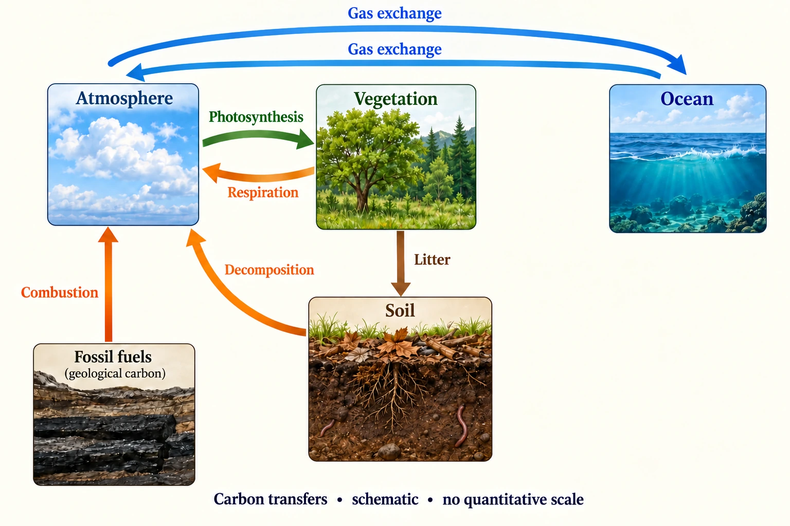
Image: illustration, not a documentary photograph. · Original generated teaching artwork; provenance retained. No, government or research-body endorsement.

10. Global carbon budgets: units, imbalance and evidence vintages

A global anthropogenic carbon budget compares fossil and land-use emissions with atmospheric accumulation and net land and ocean uptake. It does not treat the very large gross photosynthesis and respiration flows as extra anthropogenic sinks. The natural exchanges largely oppose one another; the budget concerns their net response together with human inputs. Declare the sign convention: here budget imbalance B = emissions − atmospheric increase − land sink − ocean sink. A positive B means estimated sources exceed the accounted destinations; a negative B means accounted accumulation and sinks exceed estimated sources.

The components are estimated through different methods. Atmospheric growth is constrained by concentration observations and conversion to carbon mass; fossil emissions draw on activity statistics and accounting; land-use emissions and sinks rely substantially on models and inventories; ocean estimates use observations and models. 'Observed budget' therefore does not mean every term was directly measured by a single instrument. Independent methods are useful because discrepancies expose uncertainty, but the true system still conserves carbon. A residual is not new carbon escaping conservation, and adjusting one term to force closure can hide an error.

Friedlingstein and colleagues' Global Carbon Budget 2025 was published in Earth System Science Data on 13 May 2026. The retrieved paper, accessed 4 October 2026, reports for the observation year 2024 anthropogenic source estimates of 11.6 ± 0.9 GtC/year and atmosphere-plus-land-plus-ocean partitioning of 13.3 ± 0.9 GtC/year, producing an imbalance of −1.7 GtC/year. These are dated research estimates, not 2026 measured fluxes. The authors discuss a lower alternative atmospheric-growth estimate and uncertainty in the land sink. Retain the reported imbalance rather than silently rewriting the source into perfect closure.

The paper's 2025 estimates include preliminary projections; publication in 2026 does not turn every 2025 number into a consolidated observation. Earlier preprints and later publications can differ. Pin the edition, table and units before comparing. The source has a Creative Commons Attribution 4.0 licence; attribution remains required even though the data and explanatory exercise can be reused. This lesson contains an original explanation and a small attributed numerical comparison, not a copied paper passage or a reproduced source figure.

Concentration in ppm is not an emission flux in GtC/year. Converting requires an atmospheric mass relationship and a distinction between concentration level and its change. Likewise, a remaining carbon budget for a temperature target is a cumulative allowance under specified probability and climate assumptions, whereas an annual carbon budget is an accounting of realised transfers. Confusing the two can produce the misleading claim that an annual land sink supplies a permanent additional allowance. Long-term climate effects depend on cumulative emissions and on feedbacks, not a single year's fraction alone.

Uncertainty and imbalance should make an argument more disciplined, not helpless. Evidence that budget components are uncertain does not erase a clearly positive measured atmospheric trend. Nor does one unusually weak land-sink year prove that all future uptake must vanish. Examine competing hypotheses, temporal variability and revised methods. The following closed teaching model is fictional and separate from the real 2024 comparison. Its shock isolates a mechanism so that you can predict a sign and then test whether the source observations support that magnitude; the observations cannot be used to calibrate this model without further work.

Worked example: Original fictional annual budget (GtC/year): emissions 11.5, atmospheric increase 5.3, land sink 3.2, ocean sink 3.0. In a modelled drought, the land sink weakens by 0.8 and all other inputs and ocean uptake stay fixed. Under conservation, predict atmospheric increase. Separately calculate the real 2024 reported imbalance above and a conservative bound using the two stated ±0.9 uncertainties as hypothetical hard bounds.

Evaluated extension (original task): Evaluate whether a nonzero budget residual disproves conservation or proves a new sink.

Original fictional budget closes: 11.5 − 5.3 − 3.2 − 3.0 = 0.

Drought land uptake is 2.4. If other terms stay fixed and no residual is allowed, atmosphere accumulates 11.5 − 2.4 − 3.0 = 6.1 GtC/year.

Reported real 2024 imbalance = 11.6 − 13.3 = −1.7 GtC/year. Equivalent CO2 mass = −1.7×44/12 ≈ −6.23 GtCO2/year.

For a deliberately conservative hard-bound exercise only: lowest 10.7 − 14.2 = −3.5; highest 12.5 − 12.4 = +0.1. The paper’s research uncertainties are not being relabelled as hard bounds or a confidence test.

A budget imbalance does not disprove conservation, and it does not uniquely identify an undiscovered sink. A calculated budget combines imperfect estimates of sources, reservoir changes and uptake. The Global Carbon Budget 2025 paper, published 13 May 2026, reports 2024 anthropogenic sources of 11.6±0.9 GtC/year and partitioning among atmosphere, land and ocean of 13.3±0.9 GtC/year. Their difference is−1.7 GtC/year. The authors discuss uncertainty and disagreement among estimates; these are not directly observed transfers through one perfectly measured apparatus. The publication date is not the observation year, and the paper's annual carbon budget is distinct from a remaining cumulative emissions budget.

The uncertainty exercise must preserve that distinction. The research reports uncertainties as one standard deviation. Deliberately replacing the two quoted±0.9 values with hypothetical hard bounds for a separate sensitivity exercise gives a minimum 10.7−14.2=−3.5 and maximum 12.5−12.4=+0.1 GtC/year. That envelope illustrates how permitted endpoints affect the residual; it is not a confidence test of the paper. Dependent errors and shared methods could further alter an uncertainty calculation. A residual can arise from an overestimated partitioning term, underestimated emissions or several errors together. It is insufficient evidence to choose one physical explanation without corroboration.

The separate fictional example closes exactly:11.5 GtC/year emissions equal 5.3 atmospheric increase plus 3.2 land and 3.0 ocean uptake. If drought weakens land uptake by 0.8 while the other stipulated terms stay fixed, atmospheric accumulation becomes 6.1. Reducing emissions by 1.0 in that drought scenario gives 5.1, below the original 5.3 but still positive. Concentration can therefore continue rising while gross emissions fall. The calculation explains an accounting mechanism under chosen assumptions; it does not reproduce a real drought year's measured budget or imply that ocean uptake and all other processes would actually remain unchanged.

I would treat the real imbalance as a reason to investigate estimates and mechanisms, not to force the published terms to close or to reject conservation. Independent atmospheric observations, alternative land and ocean estimates and method-specific uncertainties help assess rival explanations. Management conclusions also need a clear quantity: lower annual emissions, slower concentration growth and net concentration decline are different outcomes. The fictional transfer demonstrates that source reduction can lower the growth rate without reversing it. A persuasive geographical argument joins that mechanism to bounded evidence, reports residual uncertainty and avoids turning an annual mismatch into either a guaranteed new sink or proof that physical accounting has failed.

Answer: The fictional shock raises atmospheric accumulation by 0.8 GtC/year (about 15.1%). The real 2024 source reports −1.7 GtC/year imbalance; the artificial hard-bound envelope illustrates sensitivity, not a statistical conclusion about that paper.

Check your understanding: Transfer: in the fictional drought case emissions also fall by 1.0 GtC/year. Does atmospheric accumulation still rise? Explain why an increasing CO2 concentration need not mean emissions increased that year.

Answer: Accumulation becomes 10.5 − 2.4 − 3.0 = 5.1 GtC/year, 0.2 below the original 5.3, yet still positive. The concentration continues to rise because net inputs exceed uptake. Its growth rate can change independently of the direction of gross emissions change.

Why: Annual stock change depends on sources and sinks together. The separate source and simulation calculations preserve provenance, distinguish estimates from direct observations and avoid forcing uncertain research terms to close.