11. Coupled cycles: feedback strength, limits and thresholds

By UK A Level Geography · independent study · myAudience

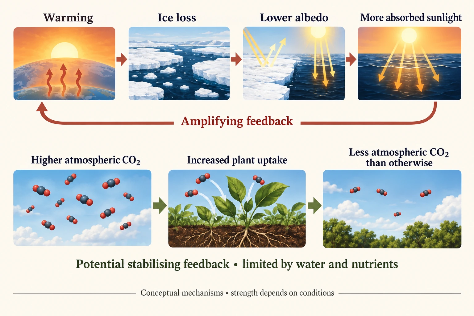
Image: illustration, not a documentary photograph. · Original generated teaching artwork; provenance retained. No, government or research-body endorsement.

11. Coupled cycles: feedback strength, limits and thresholds

Water and carbon cycles interact through vegetation, climate and ocean processes. Atmospheric CO2 affects radiative energy balance; temperature influences evaporation, soil moisture, ice and decomposition; water availability affects plant carbon uptake. A feedback loop must return to the disturbed variable. Warming followed by ice loss, reduced albedo, greater absorbed sunlight and further warming is an amplifying loop. Increasing atmospheric CO2 followed by increased plant uptake can damp the concentration rise, but only relative to the counterfactual without that uptake. Damping does not require concentrations to fall below their starting value.

The feedback plate distinguishes those two mechanisms. Its upper loop concerns reflectivity and energy, not carbon mass emitted by melting ice. Sea-ice melting changes albedo; thaw of carbon-rich soils can additionally release carbon, a separate process. The lower row depicts a potentially stabilising carbon response, limited by water and nutrients. Counted CO2 molecules and leaf sizes in the image are symbols, not measured ratios. Read 'less than otherwise' literally: it avoids implying that vegetation necessarily removes all added emissions.

Water vapour can amplify warming because warmer conditions can support more atmospheric moisture and water vapour affects outgoing radiation. Actual humidity patterns depend on circulation and supply, so the pathway is not identical everywhere. Clouds can reflect incoming sunlight and influence outgoing infrared radiation; their net response is not a universal simple sign. IPCC AR 6 (2021) assesses climate and carbon feedbacks with confidence qualifications, including uncertainty in permafrost release timing and magnitude. Those assessments are not replaced by this two-variable classroom model.

Feedback strength differs from feedback sign. A weak amplifying loop can add modestly to a disturbance; a strong loop can substantially magnify it. A stabilising loop can be overwhelmed by a continuing external input or a changing constraint. Timescale matters: rapid leaf responses, seasonal water limitation and slower ecosystem shifts can alter which feedback dominates. A threshold is a condition at which response changes qualitatively or sharply, not simply a large percentage change. For Arctic summer sea ice, IPCC AR 6 Chapter 9 assesses that stabilising winter heat-loss processes prevent a self-accelerating irreversible loss threshold in global mean temperature, despite the amplifying albedo feedback. That finding is specific to this system and assessment; it does not establish that all ice sheets or ecosystems lack thresholds. Test a proposed threshold with evidence across both sides and alternative mechanisms.

For a linear model with initial disturbance D and feedback fraction f returning each round, the total response is D/(1−f) when |f|<1. This is a geometric-series model, not a law that any climate feedback can be added numerically without attention to units and dependencies. A negative fraction in this convention alternates and damps the successive effects. If a process saturates, the fraction changes and the fixed multiplier is invalid. At |f|≥1 the infinite sum is not convergent; that mathematical failure is not proof that real Earth temperature becomes infinite.

An extended argument should couple mechanism with limits: restoring vegetation can support uptake and water regulation, but drought, disturbance and competing land needs constrain durability; fossil-emission reduction directly lowers an external input rather than relying on an uncertain compensating feedback. A claim that 'natural feedbacks will restore equilibrium' needs a timescale and equilibrium definition, and cannot guarantee that the resulting state is tolerable for people. The following values are original dimensionless scenario parameters, not estimated IPCC feedback strengths or temperature forecasts.

Worked example: Original model: an external disturbance D = 2 index units triggers feedback f = +0.25 per round. A proposed vegetation response supplies a simultaneous independent damping fraction −0.10 per round, using the same variable, timescale and normalisation. Calculate the total with and without damping. Then suppose water limitation removes damping after the first round; explain why the constant combined multiplier is no longer justified.

Evaluated extension (original task): Evaluate whether compensating natural feedbacks guarantee a tolerable equilibrium.

Without damping, total = 2/(1−0.25) = 2.6667 index units.

With both fractions constant and addable under the stated assumptions, net f = 0.15; total = 2/0.85 = 2.3529.

Reduction = 0.3137 index units, or 11.76% of the undamped total; the response still exceeds the initial disturbance of 2.

If damping applies only in the first return, that return is 0.15×2 = 0.3, then later returns use 0.25. Total = 2 + 0.3/(1−0.25) = 2.4.

Compensating natural feedbacks do not guarantee a tolerable equilibrium. A feedback returns to the disturbed variable, while its sign describes whether it amplifies or damps the initial change. The upper plate's ice–albedo loop reinforces warming by reducing reflection and increasing absorbed sunlight; it can also reinforce an initial cooling through the opposite sequence. The lower pathway describes increased plant uptake leaving less atmospheric CO2 than otherwise, not necessarily less than the initial concentration. Neither pathway establishes a measured feedback strength from the illustrated arrows, and the two mechanisms concern different physical quantities unless an explicit model relates them.

The chosen index model supplies that relationship artificially. With disturbance 2 and a constant amplifying fraction 0.25, the geometric sum is 2/(1−0.25)=2.6667. Adding a constant independent damping fraction−0.10 under the same normalization gives 2/(1−0.15)=2.3529, 11.76% below the undamped total but still above 2. If damping acts only in the first return, that first addition is 0.3 and later returns multiply by 0.25:2+0.3/0.75=2.4. The changed result demonstrates why a temporary response cannot justify the permanent combined multiplier. It is not a forecast of temperature or a calibration to IPCC feedback estimates.

Biophysical limits give reasons to question the constant fraction. Plant uptake can be constrained by water, nutrients, disturbance and changes in respiration; durable carbon storage is a separate issue from short-lived uptake. Water-vapour and cloud responses likewise require energy and circulation evidence rather than a universal sign asserted from a cartoon. IPCC's assessment that stabilising winter heat-loss processes prevent a self-accelerating irreversible threshold for Arctic summer sea ice is system-specific. It cannot be generalized to all ice sheets or ecosystems. A qualitative threshold claim requires evidence of how responses change around the proposed condition, not merely a large percentage change.

I would support restoring vegetation where evidence shows durable carbon and water benefits, while rejecting the argument that compensation makes continued external emissions harmless. Reducing an external input changes the forcing directly; relying on a response requires evidence of capacity, persistence and interactions. A mathematical equilibrium could also occur at a state that is damaging to people and ecosystems. Monitoring should therefore test both the feedback mechanism and its limits over appropriate timescales, with distributional consequences included. The justified conclusion is conditional: compensating responses can moderate change, but their existence, sign or convergence in a toy model cannot guarantee recovery to a desirable real-world state.

Answer: Constant damping gives 2.3529; one-round damping gives 2.4 under the declared revised rule. Both are conceptual indices. Neither number predicts actual warming or implies a stable climate under continuing emissions.

Check your understanding: Transfer: reverse the disturbance sign and consider ice growth and increased reflection. Does an amplifying feedback necessarily increase temperature? Explain sign and direction separately.

Answer: No. An amplifying ice–albedo loop can reinforce initial cooling: more ice reflects more sunlight and supports further cooling. Positive describes reinforcement of the initial disturbance; the disturbance itself can be negative. Magnitude depends on area, season and other energy-balance responses.

Why: The calculation and sign transfer separate causal direction, feedback sign, response strength and model scope. They prevent moral labels and unbounded geometric extrapolation from substituting for evidence.