14. Coasts as systems: sediment budgets and displaced risk

By UK A Level Geography · independent study · myAudience

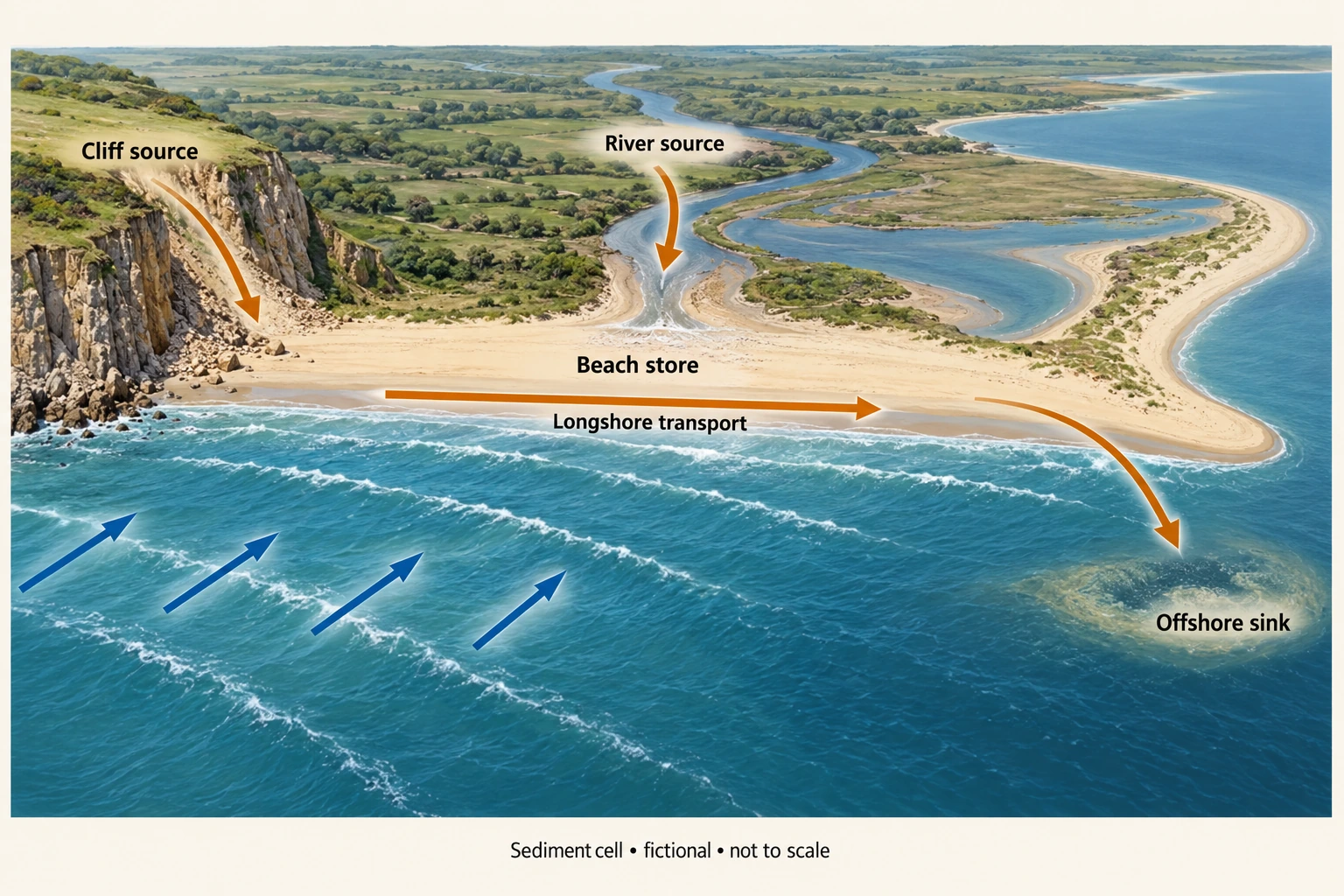
Image: illustration, not a documentary photograph. · Original generated teaching artwork; provenance retained. No, government or research-body endorsement.

14. Coasts as systems: sediment budgets and displaced risk

A coastal sediment cell is a working boundary around sources, pathways and sinks of sediment. Cliffs, rivers and offshore deposits can supply a beach; transport moves material alongshore or across the shore; deposition builds stores and erosion removes material from them. Cell boundaries may leak or shift with storms and sea-level change. As with water, a store is an amount and a flux is a transfer rate. Sand volume in m³ and dry sediment mass in tonnes cannot be added without a declared bulk density and treatment of porosity.

Winds generate waves, while tides and currents provide additional energy and transport. Waves approaching obliquely can produce swash with an alongshore component and backwash down the beach, contributing to littoral drift. Nearshore currents also transport sediment. The coast plate shows incoming blue waves and a separate orange net longshore arrow. It is fictional and not to scale; it does not claim a permanent transport direction on a real coast. Storms can reverse transport, move sediment offshore and alter beach profiles, so a single arrow is a conceptual net direction for the chosen scenario.

Weathering breaks down material in place; mass movement transfers it under gravity; marine erosion removes material and transport relocates it. Hydraulic action and wave quarrying can exploit joints; abrasion involves transported particles striking surfaces; attrition wears particles during collision; solution depends on chemistry. Cliff form also reflects rock resistance, structure, slope stability and water. A cave–arch–stack sequence is a possible developmental explanation, not a timetable through which all cliffs must pass. This lesson establishes budget reasoning but does not yet teach every required erosional and depositional landform in depth.

Groynes can trap sediment locally while reducing supply farther alongshore. A sea wall may protect assets without replacing a sediment source and can affect wave reflection and scour. Nourishment adds material but requires appropriate sediment, sourcing, monitoring and possible repetition. The sediment budget makes displaced effects visible: a gain in one beach can accompany a loss in another if the same incoming flux is redistributed. Do not treat internal longshore transport as an external output for a combined two-beach cell. The boundary decides what cancels.

The Environment Agency's current Shoreline Management Plans guidance, accessed 4 October 2026, presents planning across risks and time periods, with approaches including holding or advancing the line, managed realignment and no active intervention. A plan is a strategy, not proof that every proposed defence is funded or built. Sustainable appraisal connects cell-scale processes with assets, habitats, maintenance and unequal exposure. A coastline that is stable in one short survey interval can still have a long-term sediment deficit or episodic storm erosion.

A justified argument for protection should weigh local benefit against sediment continuity and downstream costs. For a valuable settlement, holding the line may be defensible if funding, performance and displaced effects are addressed; elsewhere, realignment can create accommodation for changing shorelines but require compensation and community involvement. The original numerical cell below uses fictional annual volumes. Its conservation check tests whether the intervention creates sediment in the analyst's accounting. It is not evidence for any real shoreline plan, and the required local and contrasting non-UK coastal cases remain outstanding.

Worked example: Original two-beach model, m³/year: external input to A=12,000; transport A→B=9,000; A offshore loss=2,000. B receives an extra river input 2,000 and loses 10,000 to an external downdrift sink. A groyne reduces A→B to 5,000 with other fluxes unchanged. Calculate each beach and combined change before/after. How much nourishment at B would prevent its new deficit?

Evaluated extension (original task): Evaluate whether protecting beach A solves the sediment problem for the whole coast.

Before: A change=12,000−9,000−2,000=+1,000; B=9,000+2,000−10,000=+1,000 m³/year.

After: A=12,000−5,000−2,000=+5,000; B=5,000+2,000−10,000=−3,000.

Combined change is+2,000 in both cases: external inputs 14,000 minus losses 12,000. Internal A→B cancels.

Nourishment of 3,000 m³/year at B makes B nominally balanced. It is a new external input with sourcing costs, not sediment created by the groyne.

Protecting beach A does not necessarily solve the sediment problem for the whole coast. Before the groyne, A receives 12,000 m³/year, transfers 9,000 to B and loses 2,000 offshore, giving a 1,000 gain. Beach B receives that 9,000 plus 2,000 from its own river input and loses 10,000 to the external downdrift sink, also gaining 1,000. The combined 2,000 gain is determined by 14,000 external inputs minus 12,000 external losses. The A-to-B transfer cancels across the combined boundary. Treating it as another external loss would obscure the difference between redistribution and a changed whole-cell supply.

Reducing the internal transfer to 5,000 raises A's gain to 5,000 but changes B's balance to−3,000. The combined gain remains 2,000: no new sediment was created by the groyne under these fixed assumptions. Adding 3,000 m³/year nourishment at B would make its nominal budget zero, but that is a new external input whose source, transport and environmental costs require consideration. A photograph of a wider protected beach cannot establish that the intervention produced a cell-wide improvement. It could instead show retention at one location paired with a downdrift deficit that emerges over a different timescale.

Real coastal management further complicates the fixed-flux illustration. Storms can change offshore export, sediment availability and the timing of redistribution; surveys need comparable datums and methods. A negative measured result after nourishment should be retained and investigated rather than removed merely because it conflicts with the model. The plate's incoming-wave orientation is consistent with the depicted rightward littoral transfer, but its arrows carry no numerical volume. Environment Agency shoreline management plans describe management approaches and investment choices dependent on evidence and funding, not a guarantee that an identified structure has been built or will keep a beach unchanged.

I would assess a groyne through cell-wide sediment and risk evidence, rather than A's volume alone. Monitoring should include repeated georeferenced profiles, storm conditions, nourishment quantities and relevant downdrift stores, with uncertainty and ecological consequences reported. Retaining sediment at A may be justified where benefits exceed costs and mitigation protects B, but affected communities should be included in evaluating the distribution. If new external losses or shifted pathways emerge, the intervention assumptions need revision. The defensible conclusion is that a local gain can be genuine while the overall sediment budget stays unchanged and another beach loses; sustainable management requires addressing that displacement explicitly.

Answer: The groyne redistributes 4,000 m³/year of retention from B to A without changing the combined budget. Preventing B’s nominal deficit requires 3,000 m³/year of additional supply under these fixed assumptions.

Check your understanding: Transfer: if the observed volume at B still falls after that nourishment, identify two possible explanations and a useful monitoring design. Should the negative observation be removed as an outlier?

Answer: Offshore losses or external export may have risen during storms, or survey/bulk-density errors may affect comparable volumes. Repeat georeferenced profiles and cell-wide surveys with consistent datum, timing and uncertainty; record nourishment and storm conditions. Retain and investigate the result, since the fixed-flux model may be wrong.

Why: A local gain and a combined-system gain are different claims. The budget evaluates causal displacement and recognises that model inputs are hypotheses vulnerable to new observations.