15. Sea level, timescale and coastal attribution

By UK A Level Geography · independent study · myAudience

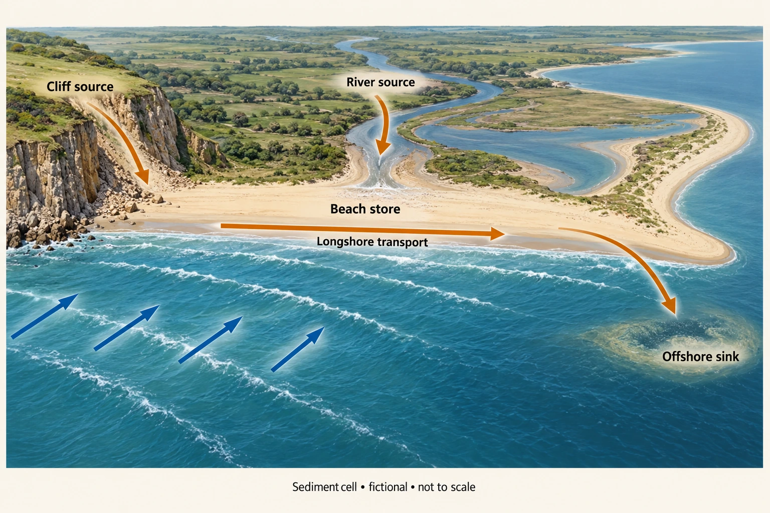
Image: illustration, not a documentary photograph. · Original generated teaching artwork; provenance retained. No, government or research-body endorsement.

15. Sea level, timescale and coastal attribution

Relative sea level is the height of the sea surface compared with local land. It can rise because water level increases, land subsides, or both; uplift can offset a sea-surface rise. Eustatic change concerns global ocean-level change, while isostatic adjustment and tectonic movements affect land. Thermal expansion raises ocean volume without requiring extra water; melting land ice transfers water into the ocean. Floating sea-ice melt has a different direct displacement relationship and is chiefly relevant here through feedbacks, not as the main direct source of global rise.

IPCC AR 6 Working Group I Chapter 9 (2021), accessed 4 October 2026, assesses global mean sea-level rise over 1901–2018 as 0.20 m with a 0.15–0.25 m range and high confidence. It also reports a much faster rate for 2006–2018 than the early twentieth-century rate. The assessed global mean is not a local tide-gauge reading and not a 2026 forecast. Its range reflects an assessment, not a classroom hard-bound instrument error. State the measurement interval and reference when quoting sea-level change; a level, cumulative change and rate are distinct quantities.

Longer coastal histories include emergence and submergence, changes over the last 10,000 years and landscapes inherited from earlier processes. Raised beaches can indicate relative emergence; drowned river valleys form rias, while fjords involve glacially excavated valleys later inundated. Landform evidence needs geological and chronological context. A raised feature alone does not locate the timing or cause precisely. This first lesson introduces those distinctions and leaves detailed located histories, tectonic cases and each required landform for later teaching.

Erosion, flooding and shoreline retreat are linked to relative sea level but also to waves, storm surge, sediment supply, geology and human intervention. A linear shoreline-retreat rule based solely on annual sea-level rise ignores those controls and can mislead. Extreme coastal water level combines mean level, tide and surge with wave effects; coincidence matters. A higher mean level can increase the frequency of threshold exceedance even without a change in storm frequency. Compare distributions rather than inferring every event was caused by one long-term trend.

The coast plate supports identification of beach and cliff stores and potential pathways but contains no elevation datum, measured retreat rate or real map. It cannot be used to measure flood depth or choose a safe development setback. Local analysis needs a common vertical datum, land-motion evidence, time-series water levels, topography and sediment information. Changing survey methods can mimic a trend. Spatial aggregation may hide one neighbourhood's exposure, and assets or vulnerability can change even where physical hazard statistics stay similar.

A justified planning argument combines adaptation to local relative change with sensitivity to uncertainty. Flexible staging and monitoring may be appropriate where exact timing is uncertain, while irreversible investment requires scrutiny of risk distribution and long-term maintenance. A national strategy cannot substitute for site evidence. The original rate model below isolates sea motion from land motion, using millimetres per year under constant-rate assumptions. It is not a projection for a named coast or an extrapolation endorsed by IPCC.

Worked example: Fictional sites X and Y over a 30-year scenario: local sea-surface rise=3 mm/year. X subsides 2 mm/year; Y uplifts 1 mm/year. Use relative rise=sea rise−land uplift. Calculate cumulative relative change. The sea-rate hard range at X is 2–4 and subsidence 1–3 mm/year. Compare its nominal change with the separate IPCC 1901–2018 global assessed change without equating intervals.

Evaluated extension (original task): Evaluate whether global sea-level information alone is sufficient for a local adaptation decision.

X land uplift is−2, so relative rate=3−(−2)=5 mm/year; over 30 years=150 mm=0.15 m.

Y relative rate=3−1=2 mm/year; cumulative 60 mm=0.06 m.

X envelope rate=2+1 to 4+3=3–7 mm/year, cumulative 0.09–0.21 m, assuming rates remain constant.

IPCC 0.20 m covers 117 years and global mean; X 0.15 m covers a fictional 30 years and local relative motion. Numeric similarity does not imply comparable rates or locations.

Global sea-level evidence is relevant context but is insufficient on its own for a local adaptation decision. IPCC's assessed 0.20 m rise, with a 0.15–0.25 m range, refers to global mean sea level over 1901–2018. The fictional site's 0.15 m change refers to 30 years and local sea level relative to moving land. Similar magnitudes do not make the rates, intervals or locations comparable. A reliable local assessment needs a consistent datum and information on vertical land motion, alongside sea-surface change. Without them, a global number can conceal whether the land itself is rising or subsiding.

The controlled scenario separates those components. AtX, sea-surface rise 3 mm/year minus land uplift−2 mm/year gives 5 mm/year relative rise and 0.15 m over 30 years. AtY, uplift of 1 mm/year reduces the relative rate to 2 mm/year and the cumulative change to 0.06 m. CombiningX's stipulated sea-rate 2–4 with subsidence 1–3 gives a 3–7 mm/year envelope, or 0.09–0.21 m. These are hard scenario bounds assuming constant rates, not a forecast distribution. Real rates can change through time, and the chosen local sea-surface term need not equal the global mean in a particular place.

Water level is also only part of coastal risk. Accelerating retreat with an apparently steady relative trend could reflect stronger storm waves, reduced sediment supply, groundwater changes or altered cliff stability. It does not automatically prove that the water-level measurements are wrong. Changes in defences can redistribute effects; sparse or inconsistent observations remain an alternative explanation to check. The coastal plate illustrates a sediment pathway, not a relative sea-level datum or actual site geometry. Adaptation decisions must therefore combine appropriately measured level trends with geomorphology, storm exposure, vulnerable assets and the expected performance of different responses.

I would use global evidence to establish the broader process, then rely on located observations and explicitly bounded scenarios for the decision. Where independent land-motion and water-level records agree and tested projections show damaging thresholds, timely adaptation is better supported. Where the dominant observed change is sediment loss or cliff instability, that mechanism requires attention alongside rising levels. Funding, habitat effects and who benefits from protection or relocation also influence a sustainable choice. The justified conclusion is neither that the global assessment is irrelevant nor that it determines one universal response: local relative change, interacting processes and distributional consequences must complete the argument.

Answer: Relative change is 0.15 m at X and 0.06 m at Y; X’s constant-rate envelope is 0.09–0.21 m. The difference between sites is caused by land motion in this controlled model, not different assumed sea-surface rates.

Check your understanding: Transfer: X’s measured shoreline retreat accelerates while relative sea-level rise appears steady. Must the water-level observations be wrong? Develop an alternative causal interpretation and test.

Answer: No. Stronger storms, reduced sediment input or a structural change in cliff stability can increase retreat despite a steady relative trend. Compare storm-wave records, sediment budgets, groundwater/geology and consistent shoreline surveys; inspect changes in defences. Multiple mechanisms can interact, and sparse sea-level sampling remains another possibility.

Why: The rate decomposition and causal transfer distinguish local relative effects from global mean change. A source interval cannot be silently replaced with a scenario interval, and a simple model cannot establish actual flood or erosion risk.