Counting language: denominators, distribution and biased samples

By UK A Level English Language · independent study · myAudience

myAudience original rendered educational illustration. Image: illustration, not a documentary photograph. · Original generated educational concept plate; retained generation provenance; no third-party text or logos.

Counting language: denominators, distribution and biased samples

A corpus is a selected collection of language evidence, not a transparent copy of everything a population says. Begin with a question and define the unit being counted. Here a token means a word token under a declared coding convention; an instance means one occurrence of our chosen fictional feature. Real work also needs decisions about contractions, punctuation, ambiguous forms and annotation. Consistent definitions make comparison interpretable; they do not remove sampling bias. For the chosen exercise, define a feature instance as the standalone token please, matched without regard to letter case; count each occurrence once. Token totals and counts are stipulated fictional data, not a supplied raw corpus or an executed search.

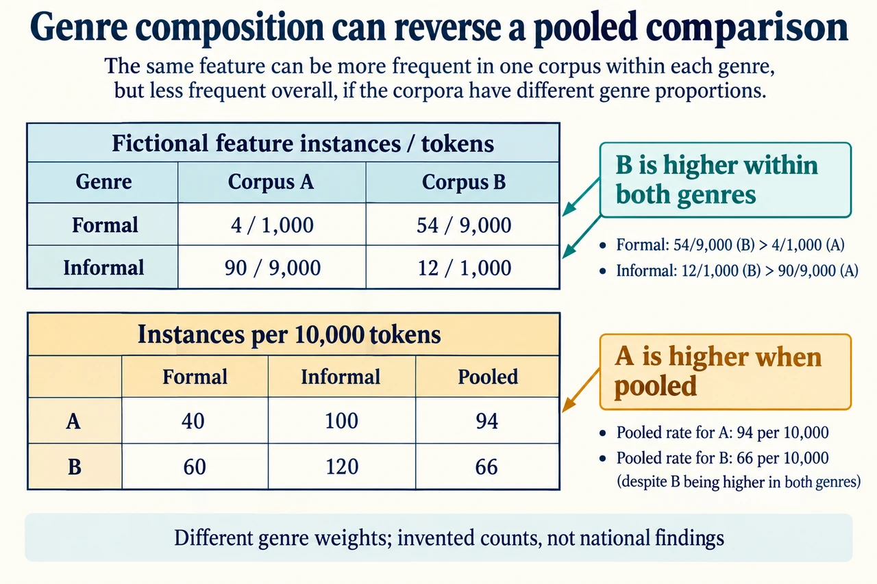
Our complete invented dataset has two corpora, each with 10,000 tokens. A contains 4 feature instances in 1,000 formal tokens and 90 in 9,000 informal tokens. B contains 54 in 9,000 formal tokens and 12 in 1,000 informal tokens. All four counts and denominators are chosen teaching numbers, not queries from the BNC, a national survey or actual social-group findings. They are designed to expose how composition can change a conclusion.

Normalise within each genre by dividing instances by tokens and multiplying by 10,000. A formal becomes 40 per 10,000; A informal becomes 100. B formal becomes 60; B informal becomes 120. B is higher in both genre comparisons. These are frequencies of a defined feature within chosen token samples, not percentages of people who use it, measures of ability or probabilities of a speaker belonging to a group.

Pooling gives A 94 instances in 10,000 tokens and B 66 in 10,000, reversing the comparison. A contains much more informal language, where the feature is more frequent in both corpora; B contains much more formal language. The difference in weights can outweigh the within-genre differences. A pooled result is not an arithmetic mistake, but it answers a different question from a matched within-genre comparison.

Under a deliberately chosen equal 50/50 genre weighting, A’s standardised frequency is (40 + 100) / 2 = 70 per 10,000 and B’s is (60 + 120) / 2 = 90. This removes the unequal genre mix for that calculation. The equal weights are an analytic choice, not a discovered population distribution. Standardisation does not correct unmeasured topic, speaker, time or selection differences, and it should not be described as making the corpora universally representative.

Distribution across texts also matters. If all 94 A instances occur in one document, a pooled rate cannot show that the feature is widespread. Repeated tokens within the same text or speaker are not automatically independent observations. Inspect lengths, counts and dispersion across relevant units, and examine the contexts of occurrences. A keyword count alone might merge unrelated meanings or misclassify a quoted feature as the writer’s own usage.

A better inquiry matches sampling to its question. Decide which genres, dates and contexts are relevant, document inclusion criteria and limitations, and check ambiguous coding with a transparent procedure. Brezina, Hawtin and McEnery’s 2021 corpus-design paper distinguishes questions a collection can address from those it cannot, and discusses several sampling biases. Our calculation illustrates that methodological issue; it does not reproduce their corpus data, licensing permissions or empirical findings.

The plate keeps counts and denominators together, then uses a second table to separate within-genre and pooled normalised frequencies. Its callouts make the reversal explicit without a misleading population ranking. Read the fictional-data label before interpreting the numbers. The illustration and worked answer explain composition; they do not establish causation, statistical significance or deficiency in any group. Authentic corpus analysis, wider sociolinguistic evidence and independently assessed research skills remain open requirements. Image: illustration, not a documentary photograph.

Worked example: Calculate the four genre rates and pooled rates, then evaluate the composition reversal and a common-weight comparison.

The invented dataset produces a genuine composition reversal, but its interpretation depends on which comparison is being made. The relevant unit is a feature instance per word token, not a percentage of speakers. Both corpora contain 10,000 tokens overall, yet their formal and informal components have different sizes.

For A, formal frequency is 4 / 1,000 × 10,000 = 40 per 10,000 tokens. Informal frequency is 90 / 9,000 × 10,000 = 100. For B, formal frequency is 54 / 9,000 × 10,000 = 60, while informal frequency is 12 / 1,000 × 10,000 = 120. B is therefore higher in each like-for-like genre comparison. Looking only at the raw counts would conceal some of these relationships because the denominators differ.

Pooling instead yields A’s 4 + 90 = 94 instances and B’s 54 + 12 = 66, each across 10,000 tokens. A is higher in that aggregate comparison. The reversal arises because A has a 90% informal token mix, whereas B has a 10% informal mix. Informal frequency is higher than formal frequency within both corpora, so their contrasting mixtures materially affect the totals. This does not make the pooled arithmetic false; it makes an unqualified inference from it unsafe.

Choose an equal 50/50 genre weighting as an explicit alternative model. A becomes (40 + 100) / 2 = 70 per 10,000 and B becomes (60 + 120) / 2 = 90. Using common weights restores the within-genre direction under this chosen comparison. It does not reveal the actual population’s genre distribution or remove differences in topic, period, speaker selection and coding.

Furthermore, frequency alone says little about dispersion. If A’s instances are concentrated in a single text, its pooled rate cannot establish widespread use. Independent texts, contexts of occurrence and an account of sampling would be needed before making a broader claim. Neither the original pooled result nor the standardised alternative proves a cause or supplies statistical significance.

The justified conclusion is thus conditional: B has the higher frequency within both specified genres and under equal weighting, while A has the higher rate in the supplied unequal mixtures. Explaining those distinct questions is more informative than selecting whichever number supports a preferred story about speakers.

Answer: Per 10,000 tokens, A formal/informal frequencies are 40/100 and B frequencies are 60/120, so B is higher within each genre. Pooled A 94 exceeds B 66 because their genre weights differ; common 50/50 weights instead give A 70 and B 90. These conditional comparisons do not establish dispersion, causation, significance or population preference.

Check your understanding: All 94 A instances occur in one document. Does A’s pooled rate establish widespread preference, and how should an inquiry be improved?

Answer: No. The pooled rate summarises token frequency in this chosen sample, not how broadly the feature is distributed or preferred. One document may contribute most instances because of its topic, author or repeated wording. Examine per-document counts and lengths, contexts and ambiguous coding, and identify the sampling units appropriate to the question. Match or account for relevant genres and periods, record inclusion criteria and consider dependence among observations from the same speaker or text. A common denominator or equal genre weighting does not solve these problems alone. Broader claims need suitable evidence; the fictional counts cannot rank social groups, establish causation or demonstrate statistical significance.

Why: A justified answer keeps the supplied linguistic forms and evidence exact, explains alternatives and limits, and does not invent speaker intentions, research outcomes or assessed completion.