A price cut can raise sales and reduce contribution

By UK A Level Business · independent study · myAudience

Original myAudience educational illustration. Image: illustration, not a documentary photograph. · myAudience educational illustration; no affiliation with any awarding body.

A price cut can raise sales and reduce contribution

Demand describes how much customers are willing and able to buy under specified conditions. A price change can alter quantity demanded along a relationship; changes in income, preferences, rivals or availability can shift that relationship. The fictional case holds other conditions sufficiently fixed to use a stipulated price-elasticity response. It does not supply an observed demand curve. This distinction matters because a simultaneous income change or new competitor could make a simple price-response forecast unsuitable for explaining what actually happened.

Price elasticity of demand compares a percentage quantity change with a percentage price change. Using the base-period convention in this case, a minus-one-point-five elasticity multiplied by a minus-ten-per-cent price change predicts a plus-fifteen-per-cent quantity change. The signs record the stipulated opposite movement. Elasticity’s magnitude helps classify responsiveness, but it is not a physical law guaranteeing the same value over every price range. Do not silently replace base-period percentages with a midpoint calculation: the numerical convention must match the inputs and interpretation.

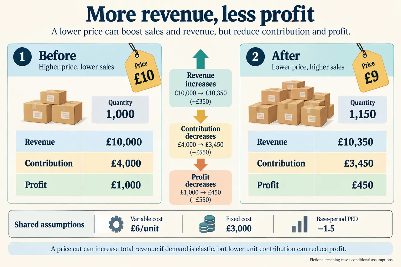
D reduces price from £10 to £9 and quantity rises from 1,000 to 1,150 under the assumption. Multiplying price by units gives £10,000 before and £10,350 after. Quantity rises sufficiently to more than offset the lower price in this revenue calculation. That result concerns receipts from sales valued at their prices, not the resources consumed supplying them. An elastic response can therefore support the claim that revenue rises while leaving the profit question unanswered. Follow the calculation to the endpoint asked about.

At unchanged £6 unit variable cost, unit contribution falls from £4 to £3. Multiplying by quantities gives £4,000 and £3,450 total contribution. With £3,000 fixed costs in each period, simplified profit falls from £1,000 to £450. The additional sales create variable costs, and every existing sale also has a smaller contribution. Showing both effects explains why the profitable-sounding increase in volume does not rescue this proposal under the stated profit objective. The numerical result should remain tied to the assumptions about costs, capacity and units sold.

The threshold transfer makes the comparison demanding. To retain £4,000 contribution at £3 per unit, D needs 1,333 and one-third units in an algebraic model. Whole-unit sales require at least 1,334, about thirty-three-point-four per cent more than the original thousand. That is much larger than the stipulated fifteen-per-cent response. Rounding down would fail to meet the threshold. This is not a forecast that customers will buy 1,334 units, nor evidence that capacity permits them; it identifies what a conditional requirement would be.

Income elasticity compares the percentage quantity response with the percentage income change. The separate example gives minus-zero-point-four and a five-per-cent income increase, implying minus-two-per-cent quantity under its assumptions. A negative income response is described as inferior, while a positive response is normal in this terminology. Inferior is not a claim that an item is defective, unsafe or socially undesirable. The classification can depend on context and range. Do not substitute a moral judgement for a defined relationship between income and demand.

Price decisions connect objectives, target customers, costs, rival actions and the rest of the mix. A lower price might support entry or an accessibility objective while reducing immediate profit; an improved explanation of the offer might attract demand without the same price reduction. Either alternative has costs and uncertain effects. A short trial needs measures of contribution and repeat demand as well as revenue. Discounts can shift the timing of purchases or attract customers who do not return, so an initial volume rise does not settle the longer-term judgement.

The plate contrasts revenue and profit in separate before-and-after panels. Shared cost assumptions are explicit, and the decorative parcels do not represent counted observations. Its main lesson is to preserve the chain from price through quantity to contribution and fixed costs. The model rejects an automatic profit claim while identifying circumstances that could change the decision. The transfer combines a whole-unit threshold with a differently signed income response. Both require careful definitions and conditional reasoning, not memorising a rule that cheaper prices always improve performance.

Worked example: Fictional D sells 1,000 units at £10 with £6 unit variable cost and £3,000 fixed period cost. A proposed 10% price reduction is modelled with base-period PED −1.5, so quantity is stipulated to rise 15% to 1,150. Unit variable cost and fixed cost remain unchanged and capacity exceeds 1,150. All figures are conditional; no latest demand estimates. A separate income example uses YED −0.4 and a 5% income rise.

D should reject the proposed permanent price cut on the present profit objective, although a limited experiment could be justified if it is designed to learn about actual demand. The stipulated elasticity of minus one point five means that a ten per cent fall in price is associated with a fifteen per cent rise in quantity using the base-period percentage method. Price becomes £9 and quantity becomes one thousand one hundred and fifty. Revenue consequently rises from £10,000 to £10,350. This supports the narrow claim that the forecast price cut raises revenue.

It does not support the stronger claim that profit rises. With unit variable cost fixed at £6, contribution per unit falls from £4 to £3. Total contribution therefore falls from £4,000 to £3,450. Subtracting the same £3,000 fixed cost leaves period profit of £1,000 before the change and £450 afterwards in this simplified model. Additional volume fails to compensate for the smaller contribution on each unit. Confusing revenue with profit would hide that mechanism and lead to the wrong recommendation for the stated objective.

The judgement depends on the assumptions. The elasticity is stipulated, not estimated from an actual controlled price experiment. Rivals might respond, customers might associate a lower price with lower quality, or the promotion could mainly bring future purchases forward. Conversely, additional production might reduce unit costs through a genuinely available economy. That possibility cannot be inserted into the calculation merely because it would rescue the proposal: the case specifically holds the £6 cost constant.

A revenue or market-entry objective could justify accepting lower immediate profit, but the business would need to explain the longer-term benefit and ability to finance the change. Capacity exceeding one thousand one hundred and fifty removes one constraint, not every constraint. Staff time, inventory and service quality still deserve investigation. A non-price approach, such as improving product information for an underserved customer group, should be compared against the same objective and its own costs.

I would retain the existing price while researching demand, or use a bounded trial with an explicit contribution measure rather than revenue alone. If a defensible estimate showed a much larger lasting quantity response, the recommendation could change. Elasticity is a conditional tool for analysing response; it is not a promise that a price cut increases every financial performance measure. A reasoned answer must connect the demand mechanism to the particular endpoint asked about.

Answer: A sustained original evaluated response: apply the stated case, verify the appropriate numerical endpoint, challenge assumptions, compare consequences and justify a conditional decision. No guaranteed business success or official mark/grade is asserted.

Check your understanding: Find the quantity at £9 needed to preserve original £4,000 total contribution with unit variable cost £6. Then interpret YED −0.4 with a 5% income rise; why does the label inferior not mean defective?

Answer: £4,000/£3=1,333.33 units, so at least 1,334 whole units are needed to meet or exceed that contribution in this model, assuming capacity/cost conditions. That is about 33.4 percent whole-unit growth, greater than 15 percent. The stipulated income example predicts −0.4×5%=−2% quantity. Inferior describes falling demand as income rises within the assumed context, not product safety, quality or social worth.

Why: Use the exact stipulated inputs, period, units and denominator; recalculate before judging. Distinguish supported conditional arithmetic from demand, causation, ethics or legal arrangements that the case does not establish.