Break-even is a boundary, not a guarantee of cash

By UK A Level Business · independent study · myAudience

Original fictional profit/cash illustration. £30−£18=£12 unit contribution; £6,000/£12=500 break-even units; 600 sales gives 100-unit safety and £1,200 simplified profit. £18,000 revenue splits into £15,000 current receipts and £3,000 received later. Opening £500+receipts £15,000−outlays £16,800=closing−£1,300. This is a timing model, not an accurate break-even graph or real accounting record.

Original myAudience educational illustration. Image: illustration, not a documentary photograph. · myAudience educational illustration; no affiliation with any awarding body.

A break-even model asks how much activity is needed for revenue to cover the costs included in a defined period. It does not predict demand or settle every cash question. Fixed costs remain unchanged over the stipulated range, while variable costs change with output or sales activity. The case assumes output is sold with no inventory change, making the production and sales quantities equal for its calculations. Outside that assumption, producing an item and receiving a customer’s payment are separate events with potentially different timings.

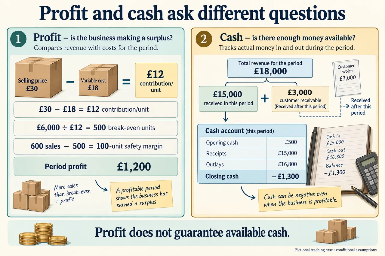
E’s price is £30 and variable cost £18 per unit, leaving £12 unit contribution. Contribution first helps cover £6,000 fixed period costs; any remaining amount produces profit in the simplified model. Dividing £6,000 by £12 gives five hundred units at break-even. At that quantity, revenue is £15,000 and variable costs are £9,000, so the £6,000 difference exactly matches fixed costs. This cross-check explains the division. Contribution per unit is not itself the final profit per unit when fixed costs remain to be covered.

Planned sales of six hundred units produce £18,000 revenue, £10,800 variable costs and £6,000 fixed costs, giving £1,200 simplified profit. Six hundred minus five hundred leaves a one-hundred-unit margin of safety. That buffer indicates how far sales could fall under unchanged model conditions before the profit becomes a loss. Capacity of six hundred and fifty is a different limit: the ability to produce does not establish customers’ willingness to buy. Neither a safety margin nor spare capacity guarantees that all the model’s conditions will continue to hold.

A chart of this model would place quantity on the horizontal axis and money on the vertical axis, with fixed cost horizontal, revenue rising from zero and total cost beginning at fixed costs. Their intersection identifies break-even. Changes in price or unit costs change the relevant slopes; changed fixed costs shift the cost level. Our illustrative calculation plate does not claim to demonstrate accurate graph construction or amendment. Those assessed skills remain open for later explicit work with verified axes, scales and coordinates, rather than being closed by decorative lines around an equation.

The model assumes constant price and unit cost within the range, known fixed costs and the stated sale of output. Discounts, overtime, capacity steps or unsold inventory can alter the relationships. In the downside case of 480 sold units, contribution is £5,760, leaving a £240 loss after fixed costs. The margin is negative twenty units relative to break-even. This sensitivity reveals vulnerability to a particular change, but does not quantify every risk. A forecast can be useful for comparing consequences while remaining dependent on uncertain inputs.

Cash timing asks when money actually enters and leaves. Of E’s £18,000 revenue, £3,000 is received only after the period, leaving £15,000 current receipts. With £500 opening cash and £16,800 cash-paid operating outlays, closing cash is minus £1,300. A customer receivable is an amount due, not cash already available to settle a supplier’s bill. The profitable £1,200 result and negative £1,300 cash forecast therefore answer different questions. Keep the delayed amount outside current receipts instead of counting it in both periods.

A deposit, earlier payment incentive, appropriate short-term finance or revised expenditure timing could address a gap, but each needs investigation. Customers may resist earlier payment; finance adds conditions and costs; extending supplier terms may damage relationships or be unavailable. The revised forecast should include any new cost and actual agreement. It is insufficient to say that credit exists somewhere and therefore the shortfall is solved. Judge the timing response together with its effects on contribution, demand and responsibilities to other stakeholders.

The worked judgement combines demand evidence, contribution and cash arrangements before recommending commitment. In the transfer, reducing price to £28 with the same £18 variable cost gives £10 contribution, making break-even six hundred units and planned profit zero. The earlier £1,200 result cannot be carried into that new case. The plate’s separate profit and cash panels preserve periods and distinguish the £3,000 receivable. Learning the formulas is a starting point; using them consistently to test a changed proposal is the more demanding decision skill.

Worked example: Fictional E sells one product for £30 with £18 unit variable cost and £6,000 fixed period cost. Planned production and sales 600 units, capacity 650. Assume units produced are sold, constant price/cost, no inventory change, tax, depreciation or financing. £3,000 of sales receipts are delayed beyond the period; all £16,800 operating cash outlays are paid in the period and opening cash £500. A demand downside case has 480 units with same price/unit cost/fixed cost.

E should not proceed with the planned trading period without a credible cash arrangement, even though its central operating model shows a profit. Each £30 sale contributes £12 after the £18 unit variable cost. Dividing £6,000 fixed costs by £12 gives break-even output of five hundred units. Planned sales of six hundred units provide a margin of safety of one hundred units and total contribution of £7,200. The resulting simplified period profit is £1,200 after fixed costs. This calculation is useful, but answers a profitability question rather than every financing question.

The plan relies on selling all output at an unchanged price and unit cost. Available capacity of six hundred and fifty units means the business can produce the planned quantity within the stipulated limit; it does not establish that customers will buy it. If sales fall to four hundred and eighty units, contribution is £5,760 and the period result becomes a £240 loss. Output is then twenty units below break-even. That sensitivity matters because the planned safety margin is a forecast buffer, not an insurance policy against every change in demand or costs.

Cash timing creates a separate problem. Six hundred sales yield £18,000 revenue, but £3,000 is not received until after the period. Cash inflow is therefore £15,000. All £16,800 operating outlays are paid within the period, and opening cash is only £500. The forecast closing cash is negative £1,300. The outstanding customer balance helps explain the difference between revenue and receipts; it cannot itself pay a bill before it is collected. A profitable period can therefore still have a funding shortfall.

E could negotiate earlier receipts or a deposit, seek suitable short-term finance, or adjust payment timings and expenditure. Each option has costs and consequences. A deposit may deter customers; extending supplier terms can strain relationships; borrowing creates repayment and possible financing costs omitted from this simple profit model. It would be misleading to recommend any of them as a costless solution. Changes must also be reflected in a revised forecast, rather than being asserted after the calculation.

My recommendation is to verify demand and resolve the cash shortfall before committing all planned expenditure. If a dependable arrangement covers the timing gap without undermining contribution or supplier reliability, six hundred sales could support the stated profit objective. If those conditions are absent, the positive £1,200 forecast does not justify proceeding unchanged. Break-even analysis identifies a conditional output boundary; combining it with cash evidence produces a more defensible decision.

Answer: A sustained original evaluated response: apply the stated case, verify the appropriate numerical endpoint, challenge assumptions, compare consequences and justify a conditional decision. No guaranteed business success or official mark/grade is asserted.

Check your understanding: If price falls to £28 with variable cost £18 and fixed cost £6,000, recalculate break-even and planned 600-unit profit. Can unchanged 650 capacity or the earlier positive profit prove adequate cash?

Answer: Contribution becomes £10/unit; break-even becomes 600 units. At 600 sales the simplified profit is zero and safety zero; capacity 650 does not guarantee sales or receipts. Recompute cash using revised revenue, credit timing and actual outlays. The old £1,200 profit forecast belongs to the old £30 price and cannot be retained. A new credit arrangement is not established merely by changing price.

Why: Use the exact stipulated inputs, period, units and denominator; recalculate before judging. Distinguish supported conditional arithmetic from demand, causation, ethics or legal arrangements that the case does not establish.