Energy balance: a boundary before a temperature

By UK A Level Environmental Science · independent study · myAudience

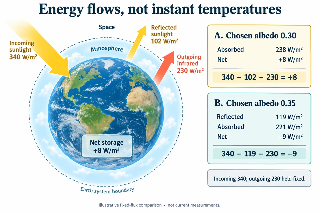
myAudience original educational concept illustration. Image: illustration, not a documentary photograph. · Original generated educational concept plate with retained actual prompts, receipts and rejected predecessors; no third-party logos or measured data.

Energy balance: a boundary before a temperature

An environmental explanation begins by drawing a boundary. For climate, one useful boundary surrounds the whole Earth system at the top of the atmosphere. Sunlight crosses inward; reflected sunlight and emitted thermal infrared cross outward. Redistribution between ocean, land and air matters greatly, but those internal transfers do not create additional energy. A different boundary around a soil surface would need a different budget, including conduction and evaporation.

Solar radiation and terrestrial thermal radiation differ in their wavelength distributions. Reflection returns part of incoming sunlight without that portion heating the system. Absorption transfers energy into matter, while emission carries energy outward. Atmospheric gases and clouds affect these paths in different ways. A greenhouse explanation therefore needs both absorption and emission; a blanket picture that blocks every outward photon cannot explain continued heat loss to space.

The familiar global incoming value is an average across the spherical surface and through time. It is not the sunlight falling on every square metre at midday. NASA’s 2009 educational account explains the geometric distinction and the uncertainty in estimated energy flows. Our illustration uses deliberately chosen rounded fluxes rather than presenting its numbers as current satellite measurements or an exact historical budget.

Choose incoming power density of 340 W/m² and a reflected fraction, or albedo, of 0.30. Multiplication gives reflected 102 W/m² and absorbed 238 W/m². If outgoing thermal emission is temporarily 230 W/m², net inward flux is 8 W/m². The complete external account is 340 = 102 + 230 + 8. The final term is a rate of energy accumulation, not an extra outgoing arrow and not a temperature rise of 8 degrees.

Changing albedo to 0.35 while deliberately holding incoming and outgoing fluxes fixed gives reflected 119 and absorbed 221 W/m². Net flux becomes − 9 W/m². This is a controlled short-term comparison that isolates reflection. Over time, temperatures, cloud properties and emission can change, so the calculation is not a prediction that the planet will continue losing 9 W/m² indefinitely or reach a particular temperature.

Power density must be integrated over time to find energy per area. A constant 8 W/m² for one day gives 8 × 86,400 = 691,200 J/m², or 0.6912 MJ/m². Turning this into a temperature change additionally requires a defensible heat capacity, depth and distribution of warming. Ocean mixing and delayed responses complicate that step. A budget identifies the direction of net storage under its assumptions; it does not supply every missing physical parameter.

The plate separates a yellow incoming solar arrow, a reflected solar arrow and a red thermal-infrared arrow at one system boundary. Its two accounting cards compare the chosen albedos with the same incoming and outgoing values. Arrow widths are schematic. The positive and negative net terms belong to storage change; they are not additional sources. The drawing omits internal exchanges intentionally, rather than claiming those exchanges do not exist.

A justified environmental judgment can connect a mechanism to evidence while keeping uncertainties visible. Increasing reflectivity would reduce absorption in this model, but a real intervention also affects ecosystems, regional weather, costs and who bears the consequences. Matched measurements and explicit counterfactuals are needed before claiming a particular benefit. Scientific uncertainty does not erase conservation of energy; it limits how confidently a simplified budget can support a specific policy.

Worked example: Evaluate the claim: increasing the reflected fraction from 0.30 to 0.35 instantly lowers global temperature by 17°C. Use the chosen incoming 340 and outgoing 230 W/m², then compare one-day net energy changes.

The claim confuses a change in power density with a change in temperature. I first keep the declared whole-system boundary, incoming flux and outgoing flux unchanged so that the comparison isolates albedo. At 0.30, reflected sunlight is 340 × 0.30 = 102 W/m² and absorption is 238 W/m². Subtracting 230 W/m² outgoing infrared gives a net inward flux of 8 W/m². The positive sign means energy is accumulating under the chosen conditions.

At 0.35, reflection becomes 119 W/m² and absorption 221 W/m². With the same outgoing 230 W/m², the net is − 9 W/m². The change in net flux is − 9 − 8 = − 17 W/m². That difference is physically meaningful within the controlled model, but watts measure energy per second. It cannot be relabelled 17°C. The two budgets also conserve energy:340 = 102 + 230 + 8 and 340 = 119 + 230 − 9, with signed storage included consistently.

For a chosen full day of constant flux, the first budget accumulates 8 × 86,400 = 691,200 J/m². The second loses 9 × 86,400 = 777,600 J/m². Their difference is − 1,468,800 J/m², or − 1.4688 MJ/m². The calculation compares energy changes over equal areas and durations. It does not mean the initial energy store was zero or that either sign would persist for a full day in an actual climate observation.

A temperature estimate would need the effective heat capacity of the affected system and a model of where the energy change occurs. A thin surface layer and a deep mixed ocean could experience different temperature changes for the same energy per area. Atmospheric emission also responds to temperature, and clouds can affect both reflection and infrared transfer. Holding outgoing flux fixed is useful for isolating the first effect, not for calculating the final equilibrium.

I therefore reject the claimed instantaneous 17°C fall while retaining a narrower conclusion: under the declared fixed-flux conditions, the larger albedo changes net storage from + 8 to − 9 W/m². To evaluate a real proposal I would seek measured radiative changes, uncertainties, response times and regional environmental effects. The arithmetic supports an initial energy-budget comparison, not a certified intervention or an exact global temperature forecast.

Answer: With the declared fluxes, net storage changes from + 8 to − 9 W/m², a difference of − 17 W/m². That is a power-density difference; an instantaneous 17°C temperature claim is unsupported.

Check your understanding: A different chosen system receives 300 W/m², reflects 25% and emits 220 W/m². Calculate its net flux and two-day energy change if those values remain fixed. Can you determine its temperature change?

Answer: Reflection is 75 and absorption 225 W/m², so net inward flux is 5 W/m². Two days contain 172,800 s; energy gain is 864,000 J/m² = 0.864 MJ/m². Temperature change cannot be determined without effective heat capacity and a response model; constant flux for two days is an explicit hypothetical assumption.

Why: Use the declared boundaries, units, fictional values and assumptions; evaluate alternatives and specify missing evidence. These original practice tasks do not establish independent assessed mastery or first-hand practical completion.