Population change: the same total can hide different pressures

By UK A Level Environmental Science · independent study · myAudience

myAudience original educational concept illustration. Image: illustration, not a documentary photograph. · Original generated educational concept plate with retained actual prompts, receipts and rejected predecessors; no third-party logos or measured data.

Population change: the same total can hide different pressures

A population count describes individuals of a defined species within a stated place and time. Changes arise through births, deaths, immigration and emigration. Each pathway has a different ecological meaning, so a total that remains constant can conceal substantial turnover. Drawing the habitat boundary also determines whether a movement is migration across the boundary or merely redistribution within it.

Birth and death affect individuals inside the population, while immigration and emigration connect it to other populations. These movements can influence recolonisation and genetic exchange as well as abundance. Habitat fragmentation may change movement opportunities, but a before-and-after count alone cannot establish the mechanism. Consistent detection methods and information about the surrounding habitat are needed to distinguish demographic change from altered observation.

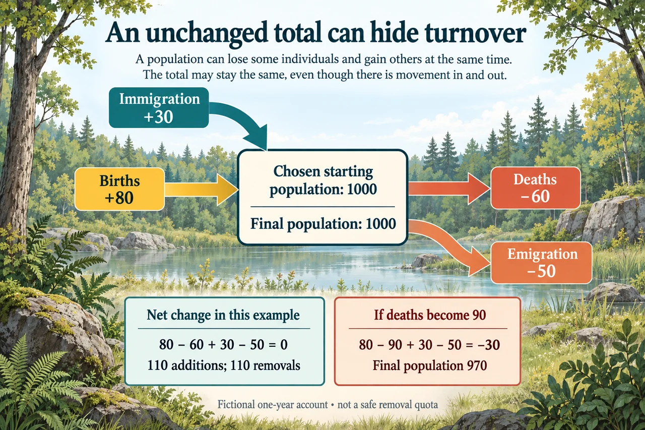
For an invented one-year account, begin with 1000 individuals, add 80 births and 30 immigrants, and subtract 60 deaths and 50 emigrants. Net change is 80 − 60 + 30 − 50 = 0, so the final total remains 1000. There have nevertheless been 110 additions and 110 removals. Calling this “no biological change” would discard the pathways and could hide a dependence on immigration or the loss of a particular age class.

Change only the chosen annual deaths from 60 to 90, keeping other terms fixed. Net change becomes − 30 and the final population 970. This calculation isolates one input; it is not a forecast that other pathways would remain fixed after a real disturbance. Food, density, disease, behaviour and habitat quality can interact with demography, so a simple accounting identity is necessary but not a complete dynamic explanation.

Abundance also differs from population structure. A stable total with fewer breeding adults may have different future reproductive prospects from one with many recruits, while a counting method may miss juveniles or hidden individuals. Repeated estimates should therefore consider detectability, age or stage composition and sampling uncertainty. A one-year arithmetic result cannot identify an exact carrying capacity or prove that a particular removal quota is sustainable.

Managing desired or undesired populations involves choices about objectives and effects on other organisms. Removing an invasive species might reduce a pressure, but collateral impacts, recolonisation and habitat conditions must be evaluated. Conversely, adding individuals does not repair an unsuitable habitat automatically. Monitoring should link the management action to the intended ecological outcome rather than treating every larger count as success.

The diagram places a chosen 1000-individual stock between four correctly directed arrows. Births and immigration point inward; deaths and emigration point outward. Their 80, 30, 60 and 50 labels refer to the same fictional interval. The unchanged 1000 endpoint is the accounting result, not a claim that the same individuals remained throughout or that the pictured habitat has a real measured population.

A defensible recommendation explains which demographic pathways are measured, which are estimated and which remain unknown. A comparison population can help evaluate other simultaneous changes, while repeated monitoring can reveal delayed consequences. Local livelihoods, animal welfare and the distribution of costs are relevant to management choices. Evidence can justify a conditional action without converting this simple balance into a universal safe harvest rule.

Worked example: A reserve manager says a fictional population that begins and ends at 1000 has “no turnover and a safe annual removal allowance of 100”. Evaluate this using births 80, deaths 60, immigration 30 and emigration 50; then compare deaths 90 with all other terms unchanged.

I first apply the population account over the manager’s chosen boundary and one-year interval. Births and immigration add 80 + 30 = 110 individuals. Deaths and emigration remove 60 + 50 = 110. The signed net change is zero, so the final count is 1000. That supports an unchanged total under the declared inputs, but it contradicts “no turnover”: additions and removals are both substantial even though they cancel numerically.

The proposed 100-individual removal allowance does not follow from this balance. No additional removal term was included in the original account. If 100 extra removals were added while every stated term stayed fixed, the net change would be − 100 and the final count 900. That is a conditional arithmetic result, not a realistic prediction of compensatory births or density effects. Such responses would require separate evidence rather than an assumed correction to the identity.

For the supplied alternative, annual deaths rise to 90 while births, immigration and emigration remain fixed. Additions are still 110, but removals become 90 + 50 = 140. Net change is − 30 and the final population 970. The result shows why an unchanged total in one interval cannot guarantee stability under changed conditions. It also does not identify the cause of the higher deaths because the task does not supply disease, food or habitat measurements.

A sustainable-management judgment would need more than one interval and a total abundance. I would examine age or stage structure, reproductive success, detection uncertainty and movement between habitats. Immigration could conceal an internal recruitment problem, while repeated emigration could reflect either normal dispersal or deteriorating conditions. Comparable observations and a defensible counterfactual are needed to distinguish these possibilities, not an invented explanation attached to the count.

I therefore accept the zero net change calculation and reject both no-turnover language and the claimed safe 100 removal allowance. The higher-death counterfactual produces 970 under the stated assumptions. The appropriate next step is to measure the relevant pathways and consequences before recommending a removal level, with attention to welfare, ecosystem effects and affected communities. The identity helps expose an unsupported inference; it does not certify a management quota or close the broader assessment of population dynamics.

Answer: The unchanged total includes 110 additions and 110 removals, so turnover is real. An extra 100 removals would produce 900 with other terms fixed, and deaths 90 instead give 970; neither account establishes a safe quota.

Check your understanding: A fictional habitat begins with 500 individuals and records 40 births, 30 deaths, 25 immigrants and 15 emigrants in one year. Calculate the final population. If immigration instead falls to 5 while other terms remain fixed, what changes, and can the count alone identify why?

Answer: The first net change is 40 − 30 + 25 − 15 = + 20, giving 520. With immigration 5 it is 40 − 30 + 5 − 15 = 0, giving 500. The count and flow data identify the arithmetic effect but not its cause; movement, habitat conditions and detection evidence would be needed.

Why: Use the declared boundaries, units, fictional values and assumptions; evaluate alternatives and specify missing evidence. These original practice tasks do not establish independent assessed mastery or first-hand practical completion.