Habitat conservation: area, edges and decisions

By UK A Level Environmental Science · independent study · myAudience

myAudience original educational concept illustration. Image: illustration, not a documentary photograph. · Original generated educational concept plate with retained actual prompts, receipts and rejected predecessors; no third-party logos or measured data.

Habitat conservation: area, edges and decisions

Protected habitat design involves more than choosing a percentage of land. Total area, internal conditions, movement routes, habitat quality and governance can affect outcomes. CBD’s current guidance on conservation networks emphasises ecological representation, connection and equitable management alongside area. These are complementary considerations: a line on a map does not ensure that a threatened population can survive or that local rights are respected.

An edge is a transition between habitats where conditions may differ from the interior. Light, wind, disturbance or movement of organisms can vary near a boundary, but the extent and ecological meaning depend on the site and species. A geometric edge-band model can compare shapes without claiming a universal ecological distance. Some organisms use edges successfully; “interior” is not automatically a value judgment about every habitat.

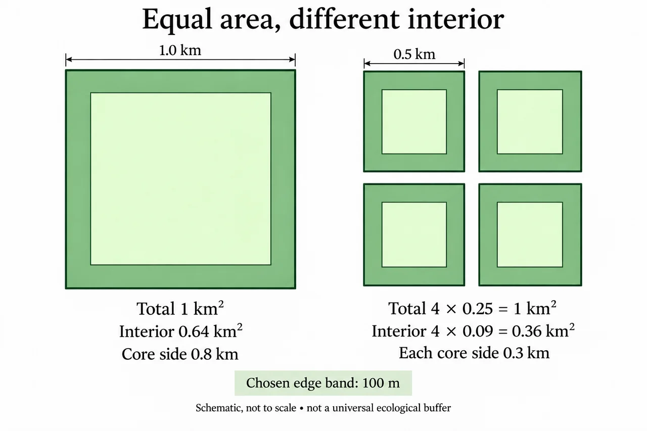
Choose a hypothetical square reserve 1 km on each side and define an interior as land at least 100 m from every edge. Subtracting 0.1 km at both ends leaves an interior side of 0.8 km. Its area is 0.8² = 0.64 km². The remaining 0.36 km² lies within the chosen edge band. This is a geometric classification, not an official legal buffer or a measured biological response.

Now divide the same 1 km² total into four separate squares, each 0.5 km on a side. Each interior side becomes 0.5 − 0.2 = 0.3 km and each core area 0.09 km². Together they contain 0.36 km² core, less than the single square’s 0.64. Extra perimeter changes the selected metric even though total protected area is unchanged. The result follows from the chosen shapes and band width, not from counting species.

Sensitivity analysis makes the assumption visible. With a 50 m band, the single square has 0.9² = 0.81 km² core, while the four squares have 4 × 0.4² = 0.64 km². The ordering remains the same, but the difference shrinks from 0.28 to 0.17 km². A decision-maker should therefore explain the origin and suitability of the band rather than use an apparently precise area to hide an arbitrary ecological threshold.

The larger continuous interior may suit one objective, while several patches might represent different habitats, spread some risks or support different communities. Connections could improve movement for a focal species yet also create routes for disturbance or invasive organisms. Decisions require species-specific evidence and the landscape context. The geometric comparison cannot by itself establish which option conserves more biodiversity overall.

The plate schematically compares one square with four smaller squares and shades the chosen edge bands. It is explicitly not to scale; use the labelled lengths, not pixel measurements, to calculate the 100 m model band and interior areas. Labels distinguish total area from interior area and mark 0.8 km versus 0.3 km interior sides. The gaps between small squares are schematic separation, not measured corridor distances. The drawing illustrates a selected geometry rather than a map of a real protected area or a recommendation to relocate people.

A conservation judgment should connect the stated goal to evidence and acknowledge affected rights and livelihoods. If the goal is continuous interior habitat under the model, the larger square has an advantage. If representation or access is the priority, other evidence may change the decision. Transparent monitoring and participation help evaluate actual outcomes, while a single numerical geometry result should remain one input rather than a universal reserve-design prescription.

Worked example: A planner says four 0.5 km-side reserves are equivalent to one 1 km-side reserve because both protect 1 km². Evaluate equivalence using a fictional 100 m interior-edge band and compare a 50 m band before recommending a design.

I distinguish equal total area from equal performance on the selected interior-area metric. The large square occupies 1 × 1 = 1 km². Four smaller squares occupy 4 × 0.5 × 0.5 = 1 km² as well, so the planner is correct about total protected area. That equality does not establish equal perimeter, internal conditions, ecological representation or movement opportunities.

With the chosen 100 m edge band, I convert the width to 0.1 km and subtract it from both ends of each side. The large square’s interior side is 1 − 0.2 = 0.8 km, producing 0.64 km² core. Each small square has 0.5 − 0.2 = 0.3 km interior side and 0.09 km² core. Four such cores total 0.36 km². On this metric, the larger square has 0.28 km² more interior, despite equal overall area.

For the 50 m sensitivity test, the band is 0.05 km and the two-edge subtraction is 0.10 km. The large core is 0.9² = 0.81 km². Each small core is 0.4² = 0.16 km², giving 0.64 km² altogether. The advantage is now 0.17 km². This demonstrates dependence on the declared band, not a measured universal ecological distance. The number should not be presented as an official buffer standard or a probability of survival.

A recommendation must also match the conservation objective. If the focal species requires continuous interior conditions and the modelled band is supported by field evidence, the large square may be preferable on that basis. If the smaller sites contain complementary habitat types or protect different local populations, they could contribute representation not captured by core area. Connectivity, disturbance, management resources and the rights of affected communities can also alter the judgment.

I therefore reject unconditional equivalence while retaining the true equal-area statement. The large square provides more modelled interior under both band choices, but that alone does not prove superior overall biodiversity conservation. I would obtain site- and species-specific evidence, compare feasible connections and agree objectives with affected people before choosing. Subsequent monitoring should test those objectives rather than merely confirm that the protected percentage has increased.

Answer: Total area is equal, but modelled interior is 0.64 versus 0.36 km² at 100 m and 0.81 versus 0.64 km² at 50 m. The large square has more interior under these assumptions; overall conservation superiority still requires ecological and social evidence.

Check your understanding: A hypothetical rectangular reserve measures 2 km by 0.5 km. With a chosen 100 m edge band, calculate its interior area and compare it with a 1 km-square reserve of the same total area. Does the result identify the best real reserve?

Answer: After removing 0.1 km at each opposing edge, the rectangle’s interior is 1.8 × 0.3 = 0.54 km². The 1 km square has 0.8 × 0.8 = 0.64 km², a 0.10 km² larger interior. This compares geometry under the same chosen band only; real habitat quality, representation, movement and community rights remain unspecified.

Why: Use the declared boundaries, units, fictional values and assumptions; evaluate alternatives and specify missing evidence. These original practice tasks do not establish independent assessed mastery or first-hand practical completion.