Temperature rise after accounting for loss

By UK GCSE Physics · independent study · myAudience

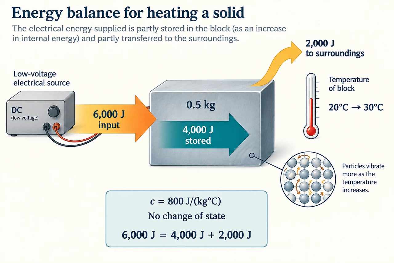
Image: illustration, not a documentary photograph. A fictional finite-interval model; energy arrows describe supplied and retained energy, not a measured apparatus result. · Original AI-generated illustration; independently reviewed scientific teaching model.

The existing energy lesson introduces the specific-heat equation. Here the challenge is deciding which energy belongs in it. For a material that remains in one phase, the thermal-energy change is E=m c ΔT, where m is mass in kilograms, c is specific heat capacity in joules per kilogram per degree Celsius, and ΔT is the temperature change. Specific heat describes the energy needed per kilogram per temperature rise. It is not the total heat capacity of an arbitrary object, and it is not energy divided by its final temperature.

A temperature interval must be formed from final minus initial temperature. Warming from 20°C to 30°C gives 10°C, not 30°C. A Celsius difference has the same numerical size as a kelvin difference, so either interval unit can be used consistently here. This does not make Celsius an absolute scale: proportional gas-temperature arguments require separate care. Within this lesson the material, phase and temperature range must be specified before treating c as approximately constant. Real values can vary with temperature and material composition.

Electrical input can be calculated from constant power and duration, Einput=P t. Watts are joules per second, so a 20 W heater running for 300 s supplies 6000 J. This input does not automatically all reach the block. If 2000 J leaves the sample boundary and no other storage term is present, the block gains 4000 J. If the heater, probe or surrounding container stores energy, that contribution must also be accounted for. A stated simplified model may omit those terms; a measured experiment cannot quietly assume them away.

Take a 0.50 kg block with c=800 J/(kg·°C), initially 20°C. In the simplified account, it stores 4000 J after the 6000 J input and 2000 J loss. Rearranging gives ΔT=E/(m c)=4000/(0.50×800)=10°C. The final temperature is therefore 30°C. The denominator 400 J/°C is the block’s heat capacity:400 J is required for each degree of warming in this model. Dimensional checking distinguishes a temperature interval from the final temperature and confirms that the result is not an energy.

Now suppose an investigator measures the 10°C rise but incorrectly assigns all 6000 J to the block. Their inferred c is 6000/(0.50×10)=1200 J/(kg·°C), exceeding the model’s true 800. The direction of bias follows from the numerator: assigning energy that escaped to the sample makes the sample appear harder to warm. This explanation does not prove that any particular real block has c=800; our numbers are an original fictional account. An independently measured or bounded loss is needed to correct an experimental estimate.

Comparisons require controlled conditions. If the same net energy is stored in two equal-mass samples, the one with lower c experiences a larger temperature rise. If masses differ or energy losses differ, that shortcut may fail. A hot drink and a cool metal handle also illustrate why temperature alone cannot tell us the total energy stored. Use the equation only for the thermal change under discussion, and avoid treating large heat capacity as a claim about safety, discomfort or every possible material property.

The illustration’s arrows form the energy account 6000 in,2000 out,4000 stored; its thermometer records 20°C to 30°C. This is a schematic and not an instruction for assembling a heater. Before accepting a calculated temperature, check phase, mass, units, net-energy boundary and whether c can be approximated as constant. Then check plausibility: positive stored energy should produce a positive temperature change in this one-phase model. If the sample reaches a phase-change temperature, the remaining energy must be treated in a separate stage.

Worked example: Find the final temperature and the bias in c if losses are ignored.

Input 20×300=6000 J.

Block gain 6000−2000=4000 J.

ΔT=4000/(0.50×800)=10°C; final 20+10=30°C.

Ignoring loss gives inferred c = 6000/(0.50×10)=1200 J/(kg·°C), 50% higher than 800.

Answer: 30°C; the loss-ignorant estimate is 1200 J/(kg·°C), 50% high.

Check your understanding: A 1.2 kg fictional solid with c=500 receives 6000 J, loses 1200 J and starts 17°C. Does it reach 27°C?

Answer: Net stored energy=6000−1200=4800 J. Its heat capacity=1.2×500=600 J/°C; ΔT=4800/600=8°C, so it reaches 25°C, not 27°C. The 27°C claim used input energy as stored energy. This answer assumes no state change, constantc and no omitted apparatus-storage term.

Why: Apply the explicit system boundary, units and model limits stated above. This original supplied transfer is not a recorded practical or completed assessment.