Testing a specific-heat estimate against its energy boundary

By UK GCSE Physics · independent study · myAudience

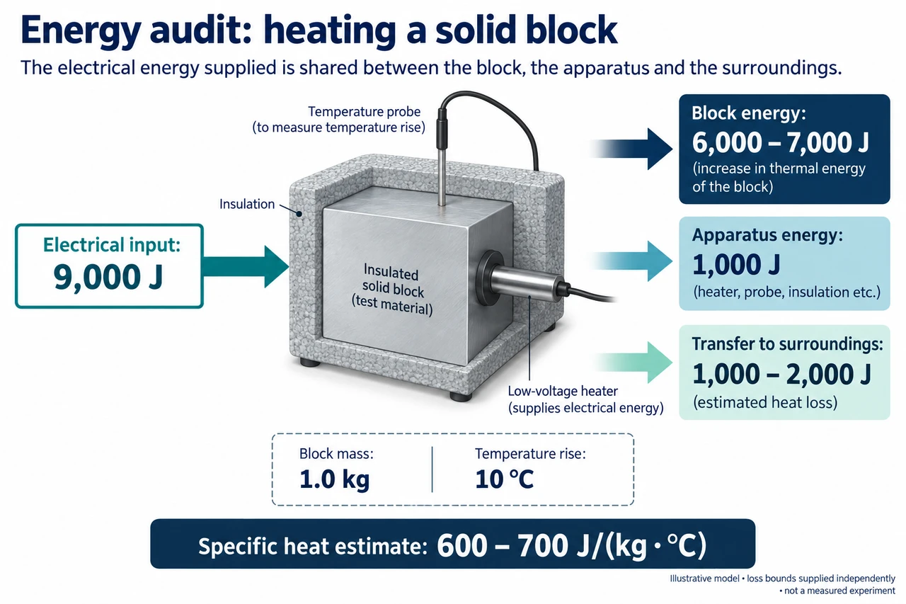
Image: illustration, not a documentary photograph. Supplied energy-account example, not a measured experiment; the 600–700 estimate uses 10°C and independently supplied loss bounds. · Original AI-generated illustration; independently reviewed scientific teaching model.

A required-practical account must explain what is measured and how a conclusion follows, rather than label a rendered setup an experiment already completed. Specific heat can be estimated from a block’s mass, its temperature rise and the energy stored in it. Electrical power and time can estimate supplied energy, but supply and sample storage need not be equal. This lesson audits that boundary. The fictional values are supplied for reasoning and do not mark the required practical, assessment or any hands-on competence complete.

A clear plan identifies the test material and mass, measures an initial temperature, monitors a known energy input and measures the resulting temperature change. A probe should sample the material meaningfully rather than an isolated hot spot. Insulation, sensible probe contact and time for temperature readings to stabilise can improve the account, but none guarantees zero losses or uniform temperature. Laboratory methods require an actual supervised risk assessment and appropriate approved equipment; this diagram does not specify wiring or a home heating activity.

For constant power 15 W over 600 s, supplied energy is 9000 J. Let a 1.0 kg block rise by 10°C. If apparatus with supplied effective heat capacity 100 J/°C warms by that same interval, its storage is 1000 J. Suppose independent evidence bounds transfer to surroundings between 1000 and 2000 J. Block storage is therefore 9000−1000−loss, giving 6000 to 7000 J. Independent means the loss estimate was not simply chosen to make the desired specific heat appear.

With the stated central 10°C interval, c=Eblock/(mΔT) lies between 6000/(1.0×10)=600 and 7000/(1.0×10)=700 J/(kg·°C). Ignoring apparatus storage and outward transfer would give 9000/(1.0×10)=900 J/(kg·°C), above both endpoints. This bias is systematic in the stated model: repeated identical mistakes do not make the result accurate. Repeating readings can reveal variation, while improved measurement of transfer and apparatus storage addresses the boundary error.

Now allow the measured temperature rise itself to lie between 9.5°C and 10.5°C. Apparatus storage changes with that interval, so it cannot remain arbitrarily fixed at 1000 J while calculating endpoints. The model is c=(9000−loss−100ΔT)/(1.0ΔT). The minimum uses largest loss 2000 J and largest interval 10.5°C:5950/10.5=566.67 J/(kg·°C). The maximum uses smallest loss 1000 J and smallest interval 9.5°C:7050/9.5=742.11 J/(kg·°C).

Outward rounding gives a conservative 566–743 J/(kg·°C) envelope for these supplied independent bounds. It is not a statistical confidence interval and does not imply a probability that the true value lies inside. Other uncertainties in mass, power, timer, temperature gradients or the apparatus model could widen or invalidate it. A relative comparison across temperatures would also need to consider whether c stays approximately constant. Reporting more decimal places cannot compensate for those omitted assumptions.

The illustration shows energy shared between block, apparatus and surroundings, with the 600–700 interval belonging specifically to the central 10°C model. It does not show the later 9.5–10.5°C extension or establish any measured loss. To evaluate a practical conclusion, inspect the system boundary, equations, units, controls, measurement quality and how uncertainty is propagated. Explain why an improvement helps, rather than adding generic instructions to repeat or insulate. The old course requirements and assessment demands remain open until real evidence demonstrates them.

Worked example: Find c from the supplied energy boundary, then propagate the temperature interval with apparatus storage consistently.

Input 15×600=9000 J.

At ΔT = 10°C apparatus storage 100×10=1000 J. Block 6000–7000 J; c = 600–700 J/(kg·°C).

Minimum(9000−2000−100×10.5)/10.5=566.666… J/(kg·°C).

Maximum(9000−1000−100×9.5)/9.5=742.105… J/(kg·°C).

Outward integer envelope 566–743, not a confidence interval.

Answer: 600–700 for central interval;566–743 conservative extended envelope.

Check your understanding: A 0.50 kg block rises 8°C. Apparatus heat capacity is 50 J/°C, input 5000 J and outward transfer 1000 J. Find c and evaluate an estimate using all input.

Answer: Apparatus stores 50×8=400 J. Block storage 5000−1000−400=3600 J. c=3600/(0.50×8)=900 J/(kg·°C). Using all input gives 5000/4=1250 J/(kg·°C),350 higher because it attributes apparatus and surroundings energy to the block. The assumed apparatus interval and outward transfer must be justified independently; the supplied fictional values are not practical-completion evidence.

Why: Apply the explicit system boundary, units and model limits stated above. This original supplied transfer is not a recorded practical or completed assessment.