Hess cycles with coefficients and states

By UK A Level Chemistry · independent study · myAudience

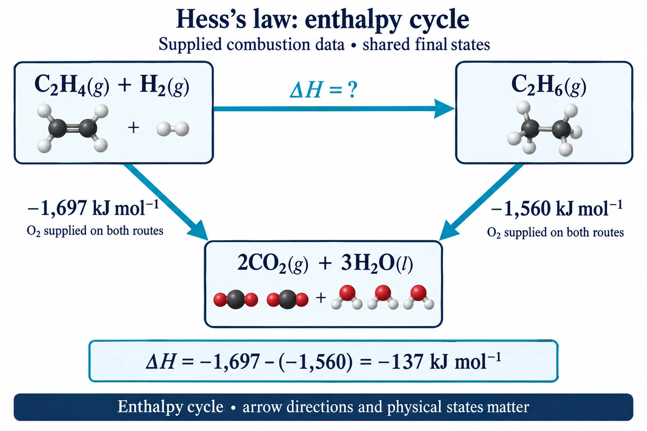
Image: illustration, not a documentary photograph. Hess route sketch with shared combustion products; oxygen is supplied on both downward routes. Arrow position is not a calibrated enthalpy scale. · Original AI-generated illustration; independently reviewed scientific teaching model.

Hess’s law lets us calculate a reaction enthalpy through other routes sharing the same initial and final states. Because enthalpy is a state quantity, adding a different path does not change the overall endpoint difference. The routes must involve the same chemical substances, amounts, physical states and conditions. A cycle is therefore an accounting structure, not a claim that every route is a feasible laboratory method. Arrows indicate equations being used forward or reversed; a misplaced arrow changes a sign.

When equations are added, intermediates cancel only if their coefficients and states match. Multiplying an equation by a factor also multiplies its enthalpy. Reversing it changes the sign. These rules make it possible to construct the target equation exactly instead of guessing a products-minus-reactants slogan for every kind of supplied data. Combustion and formation values refer to different shared endpoints, so their cycle arithmetic must follow the actual arrows. Check the cancelled equations as well as the final number.

Use supplied rounded illustrative combustion values for ethene −1411, hydrogen −286 and ethane −1560 kJ mol⁻¹, with liquid water as the relevant product state. The target is C₂H₄(g)+H₂(g)→C₂H₆(g). Both sides can reach 2CO₂(g)+3H₂O(l) when the required oxygen is included. Burning the left side releases −1411−286=−1697 kJ per mole of target reaction. Burning the right side releases −1560 kJ. The same 3.5 mol O₂ belongs to each downward route and cancels in the complete cycle.

The left downward route equals the target followed by the right downward route: −1697=ΔH_target −1560. Therefore ΔH_target=−1697−(−1560)=−137 kJ mol⁻¹. This is not simply subtracting two negative values without chemical reasoning. If the right combustion equation is reversed to connect the shared products back to ethane, its energy is +1560; adding that to −1697 yields the same target. The diagram is a route sketch, not a quantitatively calibrated enthalpy-axis plot.

A formation route provides a separate check if supplied values use identical endpoint conventions. With illustrative formation values ethane −85 and ethene +52 kJ mol⁻¹, while hydrogen in its standard state has formation value zero by definition, the target change is −85−(+52+0)=−137 kJ mol⁻¹. The rule is the sum of formation enthalpies of products minus that of reactants, weighted by their balanced coefficients. This does not mean the formation enthalpy of every element in every physical form is zero.

Physical-state mismatches require explicit corrections. If one route ends with liquid water and another with water vapour, the routes do not share the same final state until a vaporisation or condensation term is added with the correct amount. A combustion dataset and a mean gas-phase bond estimate can legitimately disagree for related reasons; averaging bond environments adds another distinction. Before treating a disagreement as a calculation error, inspect the state and condition labels, amount conventions and whether the values are measured, mean or supplied illustrative data.

The illustration has both combustion arrows pointing toward the same carbon-dioxide and liquid-water endpoint, and the target arrow connecting ethene plus hydrogen to ethane. Molecular models help identify species; the printed equations and stated oxygen addition define complete stoichiometry. To solve an unfamiliar cycle, write each supplied equation, multiply or reverse it as needed, cancel species, verify that the remaining equation is the target and then sum the correspondingly changed enthalpies. Showing that reasoning makes an answer auditable even when the final arithmetic is short.

Worked example: Calculate ethene hydrogenation enthalpy from the supplied combustion data, then check using the supplied formation data.

Left combustion total −1411−286=−1697 kJ.

Both combustion routes use 3.5 mol O₂ and share 2CO₂(g)+3H₂O(l).

Target −1697−(−1560)=−137 kJ mol⁻¹.

Formation check −85−(52+0)=−137 kJ mol⁻¹.

Reverse target changes sign to +137; twice forward gives −274 kJ for twice the written extent.

Answer: −137 kJ mol⁻¹ for the target as written.

Check your understanding: In an unfamiliar cycle A→B has supplied ΔH=+35 kJ and B→C has −90 kJ for matching amounts and states. Find C→A and two times A→C; identify a reason the arithmetic may be invalid.

Answer: A→C=35−90=−55 kJ. Reversing gives C→A=+55 kJ. Doubling the forward equation gives −110 kJ. These operations require the same intermediate B amount and physical state on both steps. If one step produces B(g) and the other consumes B(l), a phase-change term is missing, so direct cancellation is invalid. The symbols represent supplied hypothetical states, not a proposed synthesis.

Why: Use the stated equation, conservation account, units and representation limits. Supplied illustrative reasoning is not observed practical performance, completed formal assessment or evidence of mastery.