Temperature, molecular energy distributions and measured rates

By UK A Level Chemistry · independent study · myAudience

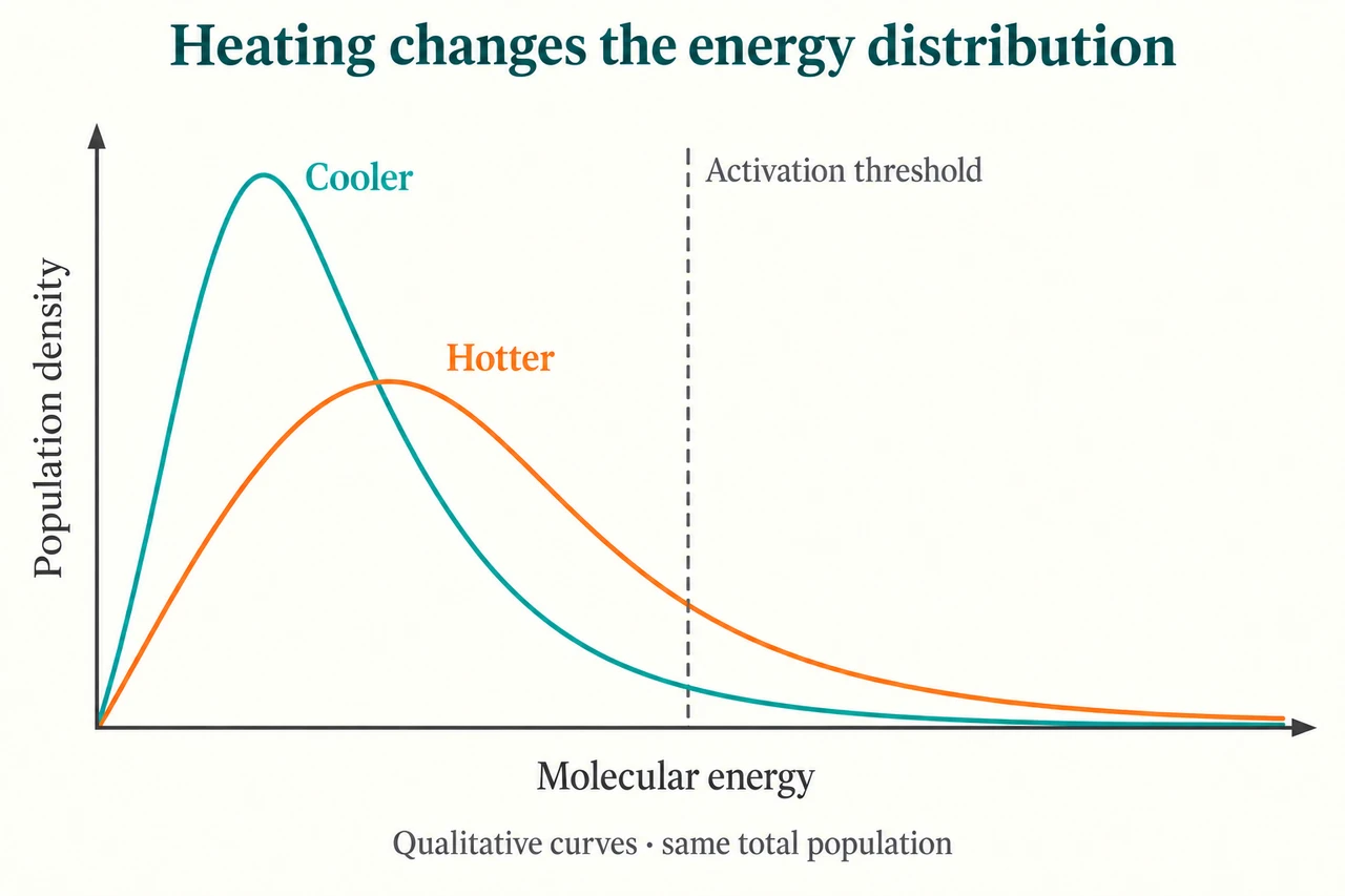
Image: illustration, not a documentary photograph. Qualitative equal-population energy distributions; heating changes the distribution while a catalyst lowers the threshold at fixed temperature. No numerical tail area or rate constant is inferred from the drawing. · Original AI-generated illustration; independently reviewed scientific teaching model.

A gas at one temperature contains particles with a range of energies. The Maxwell–Boltzmann distribution describes that spread, rather than assigning the same energy to every molecule. On the usual energy-distribution graph, the horizontal axis is molecular energy and the vertical axis is the number of molecules per energy interval, or a corresponding probability density. The area represents the total population or total probability. A smooth curve is a distribution, not a record of one molecule speeding up and slowing down. Choosing the axis meanings is essential before comparing two curves.

For the same number of gas molecules at a higher temperature, the distribution becomes broader and its peak becomes lower and moves towards higher energy. The total area remains the same. In the continuous ideal-gas energy model, the curve begins at zero at zero energy and approaches the energy axis in its long high-energy tail rather than ending at a finite maximum. The most probable energy at the peak is not the mean energy. A drawing that simply shifts an unchanged narrow curve, increases both peak and width without conserving area, or cuts off every high-energy molecule would misrepresent the comparison.

Draw an activation-energy threshold on the energy axis. The area to its right represents molecules with energy at least as large as that threshold in this simplified account. Raising temperature can substantially increase this high-energy fraction even when the change in average energy seems modest. That explains why rate can be sensitive to temperature; a small increase is not merely a tiny increase in the speed of all collisions. Energy alone is not a complete mechanism, because encounters, orientation and the reaction pathway also matter. The distribution gives an explanatory model, not an exact measured reaction rate by itself.

A catalyst lowers the threshold associated with an alternative pathway at the same temperature. It does not make the gas hotter or move the whole energy-distribution curve. More of the unchanged distribution can meet the lower requirement. Compare this with heating: temperature changes the distribution, whereas the catalyst changes which energies are sufficient for its route. A diagram should distinguish those two interventions rather than combine a moved curve and a lowered threshold without explanation. Their effects on rates can be investigated independently, while the energy endpoints and equilibrium interpretation remain separate questions.

Rate is a change in a measured quantity divided by the elapsed time for that change, with units stated. A product-gas measurement might give a mean rate in cm³ s⁻¹ over a specified interval; concentration data can give mol dm⁻³ s⁻¹. For a decreasing reactant concentration, its concentration-time gradient is negative, while the reported disappearance rate is positive. A mean over ten seconds need not equal the initial rate at zero time. An initial rate requires the local initial gradient, or a justified method that estimates it, because concentrations and rates often change as a reaction proceeds.

Suppose separate trials produce the same 20.0 cm³ of gas in 10.0 s and 6.25 s. Their interval means are 2.00 and 3.20 cm³ s⁻¹, an increase of 60%. The reciprocal-time comparison is meaningful only because the chosen extent is the same in both trials. If different volumes or different endpoints are used, comparing 1/t alone confounds time with the amount of reaction. Gas volumes also need comparable pressure and temperature measurement conditions: hotter collected gas occupies more volume for the same amount. A temperature-rate experiment must separate chemical progress from this physical measurement effect.

A useful investigation controls starting amounts, concentrations, apparatus and the chosen endpoint, measures the reaction temperature rather than relying only on the bath setting, and repeats trials to assess scatter. Delayed mixing and a subjective visual endpoint can dominate a short measured time. Suitable continuous records and a defined tangent method can improve an initial-rate estimate, but no drawing or supplied arithmetic constitutes completion of the practical study. The lesson supports planning and evaluating evidence; supervised practical work and its assessment remain open. Its illustrative distribution is qualitative, with no fitted rate constant or claimed tail percentage.

Worked example: Two supplied trials reach the same 20.0 cm³ gas endpoint in 10.0 and 6.25 s under comparable gas-measurement conditions. Find the interval mean rates and percentage increase; can the initial rates be recovered?

First interval mean: 20.0 / 10.0 = 2.00 cm³ s⁻¹.

Second interval mean: 20.0 / 6.25 = 3.20 cm³ s⁻¹.

Relative increase: (3.20 − 2.00) / 2.00 × 100 = 60%.

Endpoint equality permits the equivalent reciprocal-time ratio: (1 / 6.25) / (1 / 10.0) = 1.60.

These averages do not provide the zero-time tangents, so the initial rates remain undetermined.

Answer: Interval means are 2.00 and 3.20 cm³ s⁻¹, a 60% increase. Initial rates cannot be determined from the two endpoint times alone.

Check your understanding: A trial gives 12.0 cm³ in 8.0 s, while a second gives 18.0 cm³ in 10.0 s. Compare the mean rates and assess a claim that the slower reciprocal time proves the second trial reacted more slowly.

Answer: Mean rates are 12.0 / 8.0 = 1.5 and 18.0 / 10.0 = 1.8 cm³ s⁻¹. The second mean is 20% higher: (1.8 − 1.5) / 1.5 × 100 = 20%. Reciprocal times of 0.125 and 0.100 s⁻¹ are not directly comparable rate proxies here because the reaction extents differ. Neither pair of endpoint data establishes an initial rate or a temperature effect without controlled conditions and additional evidence. A concentration-time record and its initial tangent would be needed to estimate the initial rate; an interval average cannot supply that missing gradient.

Why: Use the stated equation, conservation account, units and representation limits. Supplied illustrative reasoning is not observed practical performance, completed formal assessment or evidence of mastery.