Reflected waves select stationary patterns

By UK A Level Physics · independent study · myAudience

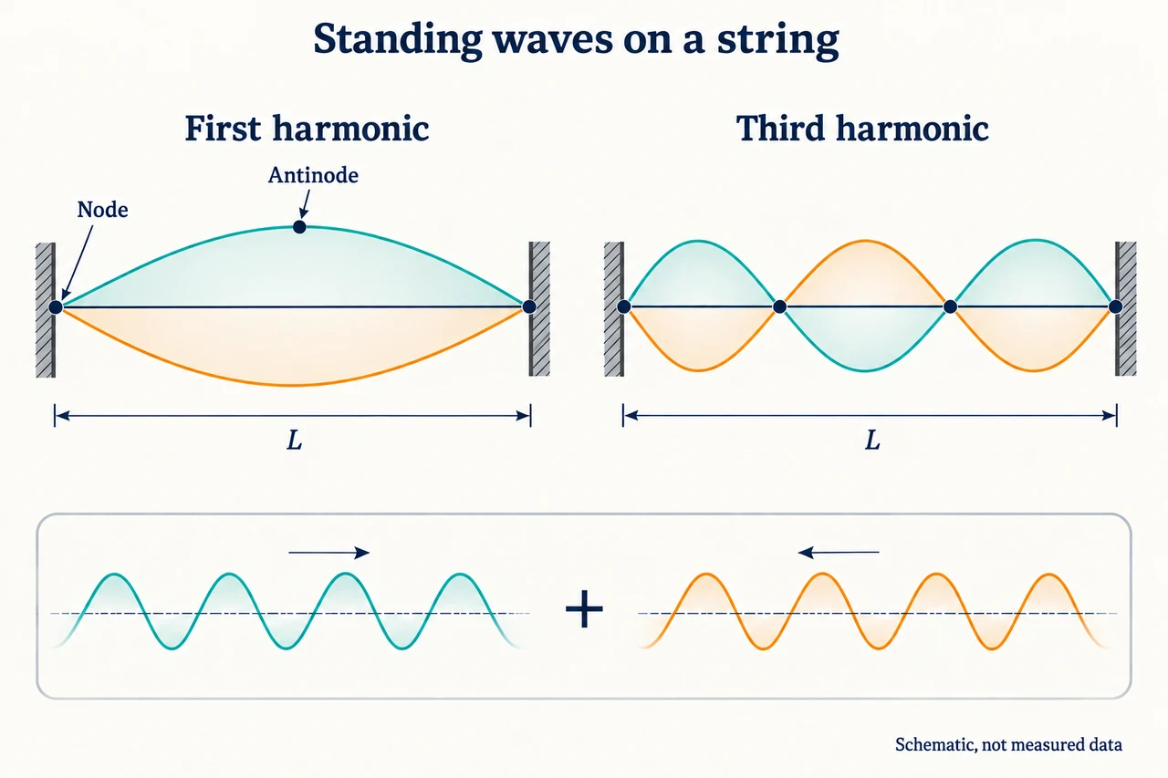
A fixed-end string supports stationary modes with nodes, antinodes and alternating adjacent-loop displacement. Selected v2 has alternate signs across adjacent third-harmonic loops. Dashed curves represent another instant, not a second physical string.

Image: illustration, not a documentary photograph. A fixed-end string supports stationary modes with nodes, antinodes and alternating adjacent-loop displacement. · Operator-authored generated illustration; scientific model and source limits reviewed separately.

A stationary wave is a pattern of oscillation that stays in place while its parts move. A stretched string can show loops with fixed positions of zero displacement, called nodes, and positions of greatest oscillation, called antinodes. The pale envelope in our drawing marks the limits reached over a cycle; it is not the string's shape at every instant. At one stage the string lies along its equilibrium line even though many points are moving through that line. Seeing zero displacement in a snapshot therefore does not establish a node. A node remains at zero displacement throughout the repeating motion under the ideal boundary conditions.

Superposition adds the displacements that individual waves would produce at the same position and time. Imagine equal-amplitude sinusoidal waves with the same frequency travelling in opposite directions. Where they always oppose, their contributions cancel and a node forms. Halfway between neighbouring nodes they reinforce most strongly at some times, creating an antinode. At other times their sum changes sign. The incoming and reflected waves continue to propagate; their superposed pattern has stationary nodes. This is not two waves colliding once and then stopping. Reflection and continued driving maintain the pattern, while real damping means energy must usually be supplied to replace losses.

Within one loop between neighbouring nodes, points oscillate in phase: they reach maximum displacement on the same side together, although their amplitudes differ. Adjacent loops oscillate in antiphase, with a phase difference of 180 degrees. The node has zero oscillation amplitude, so assigning it a meaningful oscillation phase is not useful. The distance between neighbouring nodes is half a wavelength of either component travelling wave. A stationary pattern differs from a progressive wave not merely because a picture appears still; its amplitude depends on position, and its nodes stay fixed as the local oscillations continue.

A string fixed at both ends must have a node at each end. For the first harmonic, one half-wavelength fits the length L, so λ₁ = 2 L. For the nth harmonic, n half-wavelengths fit: λₙ = 2 L/n. Combining this with v = fλ gives fₙ = nv/(2 L) when the same wave speed applies to all the modelled harmonics. The third harmonic has three loops, four nodes including both ends, and three antinodes. Counting the loops is not the same as counting interior nodes. We use first-harmonic and harmonic terminology rather than introducing overtone labels that shift the counting convention.

For an ideal flexible string at tension T and mass per unit length μ, wave speed is √(T/μ). The first-harmonic frequency is consequently f₁ = (1/2 L)√(T/μ). Here T denotes tension in newtons, not the period used in the progressive-wave lesson; each symbol must be defined locally. μ is mass divided by length in kg/m, not total string mass substituted without its length. The expression inside the square root has unit m²/s². Doubling tension multiplies frequency by √2, whereas doubling length halves frequency only if tension and μ are unchanged. These conditional comparisons are more informative than memorising a slogan about a shorter string.

A practical investigation can vary length while holding tension and μ constant, or vary tension while holding the others constant. Measuring a whole vibrating length between actual nodes is important; a support outside a node cannot automatically be used as the effective endpoint. At fixed tension and μ, a plot of first-harmonic frequency against 1/L should be linear in this ideal model. Its slope represents half the wave speed. Finding a clear resonance, reading length and assigning tension each introduce limitations. A hanging mass can approximate a tension only under stated equilibrium and apparatus assumptions. Our supplied values are teaching inputs, not a record of such an investigation.

Stationary patterns also occur with sound and microwaves. Their node labels must specify the quantity being described. In a simple sound model, a displacement node can coincide with a pressure antinode; calling both a silent point erases that distinction. A detector responding to field strength or sound pressure does not directly measure string displacement. Reflection conditions and apparatus geometry decide which patterns are supported, so the fixed-end string formula must not be copied unchanged into every tube or microwave setup. The useful shared idea is opposite-direction waves creating stable spatial variation through superposition, not an assertion that every boundary makes the same kind of node.

The first- and third-harmonic illustration uses equal endpoint separation and shows opposite snapshots inside each envelope. It should be read as a model of possible motion, not measured amplitudes. In an ideal equal-amplitude stationary wave, net progressive energy transfer averages to zero, although energy moves locally between parts and changes form during oscillation. Real driven, damped systems need continuing input. Explaining a node or calculating a resonance does not establish that a learner has safely operated a signal generator or completed the practical study. The lesson prepares that reasoning; observed apparatus competence, experimental records and assessed practical performance remain separate requirements.

Worked example: A fixed-end string has vibrating length 0.80 m, tension 57.6 N and mass per unit length 0.0040 kg/m. Determine its wave speed, first and third harmonic frequencies and third-harmonic node positions. Explain the cancellation at a node.

The boundary model requires a node at each fixed end. Keep μ as mass per unit length rather than replacing it by a total mass. T is tension here; it is not an oscillation period. Assume the string is uniform and the small-disturbance speed formula applies.

Compute v = √(57.6/0.0040) = √14400 = 120 m/s. The quotient has unit N divided by kg/m, which reduces to m²/s² before the square root. A numerical square root without this unit check could conceal a wrong input quantity.

One half-wavelength fills 0.80 m at the first harmonic, giving λ₁ = 1.60 m. Then f₁ = 120/1.60 = 75 Hz. This is also obtained directly from f₁ = (1/2 L)√(T/μ), so the geometry and speed calculation agree.

The third harmonic has λ₃ = 2 L/3 = 1.60/3 = 0.533333… m and f₃ = 3 × 75 = 225 Hz. Three loops fit the length; calling it the third harmonic does not mean three interior nodes or a wavelength three times the first.

Node separation is λ₃/2 = L/3 = 0.266667… m. Starting at the left fixed end, nodes occur at 0,0.266667…,0.533333… and 0.80 m. Antinodes lie midway between them, at 0.133333…,0.400 and 0.666667… m under this ideal geometry.

At a node the two component displacements are equal and opposite at every instant. They need not each be zero separately. Within one loop points oscillate together; across an interior node adjacent loops reverse their phase. The envelopes illustrate these boundary and phase statements rather than providing measured amplitudes.

Answer: Wave speed 120 m/s; first harmonic 75 Hz; third harmonic 225 Hz, wavelength 0.533333… m. Four nodes including both ends occur at intervals of 0.266667… m.

Check your understanding: The length becomes 0.60 m and tension becomes 14.4 N, with μ unchanged. A learner predicts a first harmonic of 100 Hz because only the shorter length matters. Find the correct first and third harmonics, explain the failed assumption, and say whether a sound pressure minimum can automatically be called a particle-displacement node.

Answer: The tension is one quarter of 57.6 N, so speed halves: √(14.4/0.0040) = 60 m/s. The new first harmonic is 60/(2 × 0.60) = 50 Hz and the third is 150 Hz. The length-only calculation 75 × 0.80/0.60 = 100 Hz wrongly holds wave speed fixed. The simultaneous tension change multiplies that result by one half. The new third-harmonic wavelength is 0.40 m, with nodes 0,0.20,0.40 and 0.60 m. For sound, pressure and particle displacement are different quantities: in the simple stationary-sound model their nodes and antinodes are interchanged. The detector's response and boundary conditions must be specified before naming a node.

Why: A parameter-change argument must retain all changed factors and identify the measured physical quantity. Reading a pressure pattern does not establish string-like displacement boundaries.