Half-life describes a population, not a countdown

By UK GCSE Physics · independent study · myAudience

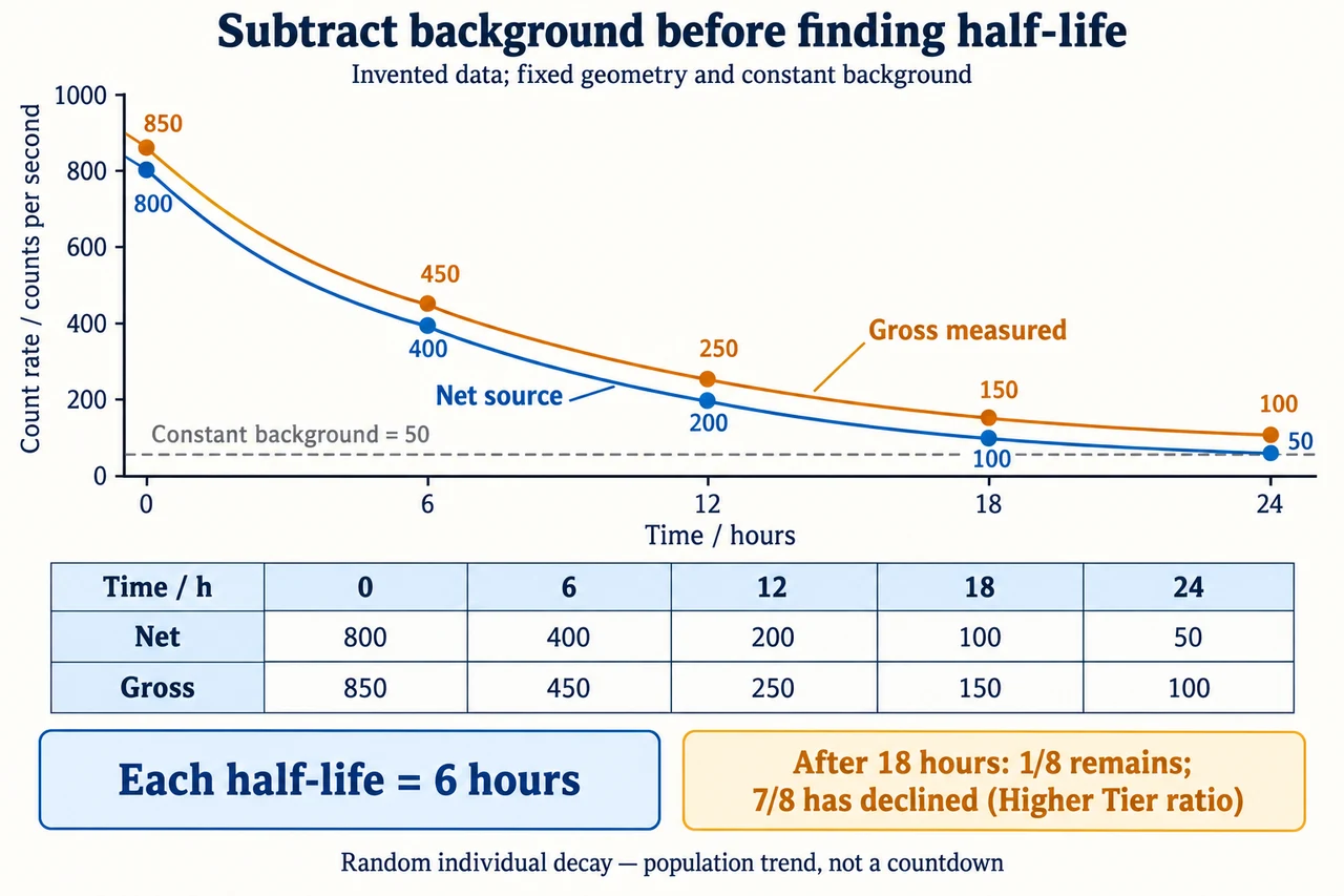
Image: illustration, not a documentary photograph. These invented data assume one isotope, fixed detection geometry and constant background of 50 counts per second. At 0, 6, 12, 18 and 24 hours the net source rates are 800, 400, 200, 100 and 50; gross measured rates are 850, 450, 250, 150 and 100. Subtract background before finding the six-hour half-life. The curves are schematic and the table coordinates are authoritative. After three half-lives, one eighth remains and seven eighths has declined; this ratio task is Higher Tier. Individual decay is random, not a nucleus countdown or a promise that every tiny sample halves exactly. Count rate is not a dose or safety criterion. The 160-pixel preview supports recognition rather than reading every graph label. · Original myAudience generated illustration; not a documentary photograph or exam-board endorsement.

Half-life describes a population, not a countdown

A radioactive nucleus does not carry a clock that tells us when it will decay. We can describe the behaviour of a population of one isotope without predicting the decay time of a particular nucleus. Half-life is the time over which that population's number of undecayed nuclei, and therefore its activity in the simple single-isotope model, falls to half. A small sample fluctuates; a large population gives a much more regular statistical pattern. Surviving one half-life does not make a nucleus due to decay in the next. Random individual events and a predictable population trend are compatible descriptions.

Track what remains, rather than subtracting the same amount repeatedly. If a large population begins at an expected 8000 undecayed nuclei, successive half-lives give expected populations of 4000, 2000 and 1000. The amount lost during each interval becomes smaller because fewer nuclei remain. After three half-lives, one eighth remains and seven eighths have decayed. These are population-model values, not a guarantee that an actual tiny sample contains a fractional nucleus or that every measurement falls exactly on a smooth curve. Calculating the net decline as a ratio is a Higher Tier extension within the GCSE specification; the definition and interpretation of half-life are shared core ideas.

Activity and detected count rate are related but are not interchangeable. Activity counts decays per second in the source, measured in becquerels. A detector records events it can detect; geometry, absorption, efficiency and the measurement system affect its count rate. A constant setup can allow count-rate changes to track the same isotope's decay without determining its absolute activity. Keep the source position, intervening material and detector response fixed when interpreting an idealised decay trend. A change in how much radiation reaches the detector can imitate a change in the source. None of the fictional data here are measurements from a radioactive specimen.

Background counts must be separated from the source signal. In our invented fixed-geometry model, measured gross rate equals source-related net rate plus a constant background of 50 counts per second. An initial gross rate of 850 therefore means a net rate of 800. If the half-life is six hours, net rates at six, twelve and eighteen hours are 400, 200 and 100; gross rates are 450, 250 and 150. The gross rate is not halved each time because the background contribution does not decay with the sample. Subtracting the background before looking for repeated halving is the essential measurement step.

A graph can reveal half-life when its quantities are interpreted correctly. Starting from net rate 800, locate the time where net rate reaches 400; in our model it is six hours. Starting instead at net rate 400 and locating 200 gives another six-hour interval. Repeating the comparison tests whether one constant half-life fits the trend. A straight line that loses 400 counts per second every six hours would become negative and is not this decay model. Gross-rate data approach their background level rather than zero. A fitted curve or clear graph does not eliminate uncertainty in individual counts or in the background estimate.

Counting for longer can reduce relative fluctuation under suitable stable conditions, but it cannot fix a changing background or a displaced detector. A measured rate is obtained by dividing recorded counts by the counting interval, so counts and counts per second must not be confused. For example, an average gross rate of 450 counts per second corresponds to 27 000 counts in a 60-second interval under the stated constant-rate approximation. The expected background contribution is 3000 counts, leaving 24 000 net counts, or 400 counts per second. Actual recorded totals fluctuate and are not required to equal these expectations.

A threshold question needs the threshold's definition. In this fictional model, reaching a gross rate of 100 means the net rate has fallen to 50. The progression 800, 400, 200, 100, 50 requires four half-lives, or twenty-four hours. It does not require three half-lives merely because 800 has fallen to 100 at eighteen hours: that 100 is a net rate, so its gross rate is 150. The distinction also prevents impossible finite-time predictions. With constant background 50, a positive source contribution cannot produce a gross rate below 50 under this ideal model. A count-rate threshold is not a radiation-dose or safety criterion.

Source and scope: GCSE Physics atomic structure, the related topic and activity/background context, checked 6 October 2026:. This lesson uses the existing the related topic source record; assessed mastery remains open. OpenStax College Physics 2e 31.5 provides an independent check of the standard statistical half-life concept: https://openstax.org/books/college-physics-2e/pages/31-5-half-life-and-activity. Its historical carbon-dating example is outside this lesson’s scope. Source reuse restrictions remain applicable; the explanations, invented data, questions and illustration here are original rather than reproductions of source material. Practical/radiological safety and full qualification assessment remain open. The reviewed illustration is schematic; its full caption explains the model and preview limits.

Half-life alone does not establish a material's hazard or a suitable use. Emission type, energy, amount of material, exposure route, shielding and other conditions matter. Different isotopes and decay chains can produce a sum of trends that is not one simple repeated-halving curve. This lesson deliberately uses one isotope, constant detection conditions and constant background. It teaches population randomness, corrected decay data and an explicitly labelled Higher Tier ratio calculation; it does not provide a source-handling procedure, a radiological safety judgement, completed practical evidence or full nuclear-physics coverage.

Image: illustration, not a documentary photograph. These invented data assume one isotope, fixed detection geometry and constant background of 50 counts per second. At 0, 6, 12, 18 and 24 hours the net source rates are 800, 400, 200, 100 and 50; gross measured rates are 850, 450, 250, 150 and 100. Subtract background before finding the six-hour half-life. The curves are schematic and the table coordinates are authoritative. After three half-lives, one eighth remains and seven eighths has declined; this ratio task is Higher Tier. Individual decay is random, not a nucleus countdown or a promise that every tiny sample halves exactly. Count rate is not a dose or safety criterion. The 160-pixel preview supports recognition rather than reading every graph label.

Worked example: An invented source has a six-hour half-life. Under fixed detection conditions, its initial gross count rate is 850 counts per second and background is constant at 50 counts per second. Give net and gross rates after 6, 12 and 18 hours. State the remaining fraction and net decline after 18 hours, and find when gross rate first reaches 100 counts per second in this ideal model. Explain why halving gross rates gives the wrong answer.

Subtract background: initial net rate is 850−50=800 counts per second. Only this source-related component follows the assumed halving model.

Six, twelve and eighteen hours are one, two and three half-lives. Net rates are 800/2=400, 800/4=200 and 800/8=100 counts per second.

Restore the background to predict gross rates: 400+50=450, 200+50=250 and 100+50=150 counts per second. The non-decaying offset explains why gross rates are not repeatedly halved.

After three half-lives the remaining fraction is 1/8. The decline is 1−1/8=7/8, so remaining:initial is 1:8 and decline:initial is 7:8. This numerical ratio task is the Higher Tier extension.

Gross threshold 100 corresponds to net threshold 100−50=50. Four halvings take 800 to 50, so the time is 4×6=24 hours. At eighteen hours the gross rate is still 150, not 100.

Answer: Net rates after 6, 12 and 18 hours are 400, 200 and 100 counts per second; gross rates are 450, 250 and 150. After 18 hours one eighth remains and seven eighths have declined, with ratios 1:8 and 7:8 respectively. The gross rate reaches 100 after 24 hours, when net rate is 50. Halving gross readings incorrectly treats constant background as decaying source signal. These expected values do not specify an individual nucleus's decay time or certify a safe exposure.

Check your understanding: Repeat the same net-source model with background 100 counts per second. What are the gross rates initially and after 6, 12, 18 and 24 hours? Can it reach a gross rate of 100 in a finite time under this ideal model? When does it reach 150? A learner also says every nucleus surviving six hours must decay during the next six hours. Explain the mistake.

Answer: The unchanged net sequence is 800, 400, 200, 100 and 50, so gross rates are 900, 500, 300, 200 and 150 counts per second. Reaching gross 100 would require net zero; the ideal smooth positive decay model approaches that background level without reaching it in a finite time. Gross 150 corresponds to net 50 and occurs at 24 hours. An actual small radioactive population can eventually lose all of its nuclei, so the smooth-model limit must not be presented as a literal guarantee about each finite sample. A surviving nucleus has no six-hour deadline: individual decay is random, and survival through one interval does not determine decay in the next.

Why: Write gross=net+background before applying any fraction. Changing only background should alter gross readings but leave the source's half-life unchanged, which is a strong check on the reasoning. The threshold subtraction also reveals whether a requested reading is reachable in the chosen model. Finally, distinguish an expected population curve from the discrete outcomes of individual nuclei: otherwise the valid repeated-halving calculation turns into an invalid countdown story.