A stiffer wire need not be a different material

By UK A Level Physics · independent study · myAudience

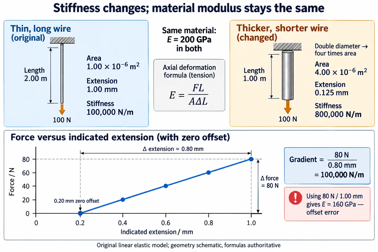
Image: illustration, not a documentary photograph. The original ideal wire has length 2.00 metres, area 1.00×10⁻⁶ square metres and extension 1.00 millimetre under 100 newtons. Halving length and doubling circular diameter multiplies area by four and reduces extension to 0.125 millimetres. Specimen stiffness rises from 100 000 to 800 000 newtons per metre, while the stipulated material modulus stays 200 gigapascals. The wire shapes are schematic, not to scale or identified real materials. The invented graph has a 0.20-millimetre indicated zero offset: its gradient is 80 newtons divided by 0.80 millimetres, whereas the uncorrected last-point ratio incorrectly gives 160 gigapascals. Formulas and labelled coordinates are authoritative. The model assumes a justified linear elastic range; no safe load, fracture property or completed practical is claimed. The 160-pixel preview supports recognition rather than reading every graph label. · Original myAudience generated illustration; not a documentary photograph or exam-board endorsement.

A stiffer wire need not be a different material

A wire's extension depends on its material and its geometry. Comparing two extensions without recording length, cross-sectional area and load can therefore produce a false material ranking. Tensile stress is axial force divided by original cross-sectional area, σ=F/A. Tensile strain is extension divided by original length, ε=ΔL/L. Stress has units of pascals; strain is dimensionless because it is a ratio of lengths expressed in the same units. Neither is simply another name for force or extension. Normalising the measurements lets us discuss material response rather than the size of the specimen alone.

In a linear elastic range, Young modulus is the stress-to-strain ratio E=σ/ε=FL/(AΔL). It is also the gradient of a straight stress–strain graph in that range. The formula requires the stated deformation model and appropriate measurements; dividing two values outside a linear range is not automatically a valid Young modulus. Elastic recovery and linear proportionality are related but distinct ideas. A material can depart from a straight proportional response before reaching a limit beyond which it fails to return to its original dimensions. Breaking stress and Young modulus answer different questions and must not be interchanged.

Our original fictional wire has length 2.00 metres and original cross-sectional area 1.00×10⁻⁶ square metres. An axial force of 100 newtons produces an extension of 1.00×10⁻³ metres, within a stated linear elastic range. Stress is 1.00×10⁸ pascals; strain is 5.00×10⁻⁴. Their ratio is 2.00×10¹¹ pascals, or 200 gigapascals. This numerical value is a stipulated specimen model, not identification of a named alloy or proof of a measured manufacturer's property. Conditions such as temperature and specimen structure can matter in real material comparisons.

Separate specimen stiffness from material modulus. For this uniform tensile model F=kΔL, where k=EA/L. The fictional wire therefore has k=1.00×10⁵ newtons per metre. A longer wire of the same material and area has a smaller stiffness, while a larger area increases stiffness. For a circular cross-section A=πd²/4, so doubling diameter multiplies area by four, not two. None of these changes requires E to change. The model assumes uniform axial loading and an appropriate effective gauge length; it does not describe bending, a loose attachment or extension dominated by the test frame.

A measurement method should determine a relationship rather than rely on one dramatic extension. Within the range being studied, obtain force and extension pairs, inspect a force–extension graph and find its gradient. Record the original gauge length and cross-sectional area independently. For a circular wire, diameter measurements at several positions and orientations help reveal variation; a small diameter error matters because area depends on its square. A fixed reference or comparison arrangement can help distinguish specimen extension from support movement, but it does not eliminate every apparatus effect. Repeated readings, unloading checks and a justified linear interval provide evidence rather than a declaration that the required practical has been completed.

Consider invented graph readings: F=0,20,40,60,80 newtons gives indicated extensions 0.20,0.40,0.60,0.80,1.00 millimetres. The 0.20-millimetre indication at zero load is an offset. The gradient from the first to last point is 80/(0.80×10⁻³)=1.00×10⁵ newtons per metre, giving E=200 gigapascals with the stated geometry. Using 80/(1.00×10⁻³) instead gives 8.00×10⁴ and E=160 gigapascals because it treats the offset as physical extension. An intercept is evidence to examine, not a licence to discard inconvenient points or force a graph through the origin. This example's offset is stipulated; a real intercept needs investigation.

The energy stored during a linear loading process is the area under the force–extension graph, U=FΔL/2. At 100 newtons and 1.00 millimetre of actual extension, U=0.0500 joules. This small value is consistent with a small extension even though the material modulus is large. The expression is not a general formula for every nonlinear loading path or for recoverable energy after plastic deformation. In an uncertainty budget, contributions from force–extension gradient, length and area also need attention. Uncertainty affects confidence in a comparison; it does not alter the algebraic distinction between stiffness and modulus.

Source and scope: mechanics and materials, the related topic Young modulus with the related topic context, checked 6 October 2026:. The specification is version 1.4, July 2026. It requires a simple measurement method and Required This practical study; this written example does not perform or complete that practical. This lesson uses two separately documented local records for Young modulus and written This practical study preparation, linked to existing official source obligations. Performed practical evidence and assessed mastery remain open. OpenStax University Physics Volume 1 12.3 provides a concept check: https://openstax.org/books/university-physics-volume-1/pages/12-3-stress-strain-and-elastic-modulus. Source reuse restrictions remain applicable; the explanations, specimen and graph models, questions and illustration here are original rather than reproductions of source material. Full materials coverage, practical endorsement and qualification assessment remain open. The reviewed illustration is schematic; its full caption explains the model and preview limits.

For a changed specimen of the same material, halve the length and double the circular diameter while retaining a 100-newton load. Its area becomes 4.00×10⁻⁶ square metres and its length 1.00 metre. The predicted extension is one eighth of the original: 0.125 millimetres. Its stiffness is eight times larger, but its stress and strain are both one quarter of the original, so E remains 200 gigapascals. The result tests whether geometry has been confused with material properties. This is an ideal linear tensile calculation, not a design recommendation, a safe-load specification or evidence that a real wire cannot fracture.

Image: illustration, not a documentary photograph. The original ideal wire has length 2.00 metres, area 1.00×10⁻⁶ square metres and extension 1.00 millimetre under 100 newtons. Halving length and doubling circular diameter multiplies area by four and reduces extension to 0.125 millimetres. Specimen stiffness rises from 100 000 to 800 000 newtons per metre, while the stipulated material modulus stays 200 gigapascals. The wire shapes are schematic, not to scale or identified real materials. The invented graph has a 0.20-millimetre indicated zero offset: its gradient is 80 newtons divided by 0.80 millimetres, whereas the uncorrected last-point ratio incorrectly gives 160 gigapascals. Formulas and labelled coordinates are authoritative. The model assumes a justified linear elastic range; no safe load, fracture property or completed practical is claimed. The 160-pixel preview supports recognition rather than reading every graph label.

Worked example: A fictional uniform wire has L=2.00 m and A=1.00×10⁻⁶ m². Within its stated linear elastic range, F=100 N gives actual extension 1.00 mm. Find stress, strain, Young modulus, specimen stiffness and stored energy. Then use the invented graph F=0,20,40,60,80 N with indicated extensions 0.20,0.40,0.60,0.80,1.00 mm to obtain stiffness and modulus, explaining the intercept error in using the last point alone.

Convert extension before dividing: 1.00 mm=1.00×10⁻³ m. Stress is 100/(1.00×10⁻⁶)=1.00×10⁸ Pa; strain is(1.00×10⁻³)/2.00=5.00×10⁻⁴, with no unit.

E=σ/ε=(1.00×10⁸)/(5.00×10⁻⁴)=2.00×10¹¹ Pa=200 GPa. The result uses the explicitly linear elastic interval and original specimen dimensions.

k=F/ΔL=100/(1.00×10⁻³)=1.00×10⁵ N/m. Independently EA/L=(2.00×10¹¹)(1.00×10⁻⁶)/2.00 gives the same stiffness.

Stored energy is half the rectangular product: U=100×(1.00×10⁻³)/2=0.0500 J. This is the triangular area under the actual linear force–extension relation.

In the graph, extension change is 1.00−0.20=0.80 mm over a force change 80 N. The gradient is 80/(0.80×10⁻³)=1.00×10⁵ N/m and E=kL/A=200 GPa. Using the uncorrected last indication gives k=8.00×10⁴ N/m and E=160 GPa; the 20% underestimate comes from counting the stipulated zero offset as extension.

Answer: Stress is 1.00×10⁸ Pa, strain 5.00×10⁻⁴, E=2.00×10¹¹ Pa, k=1.00×10⁵ N/m and stored energy 0.0500 J. The graph's gradient reproduces this stiffness and modulus. Its nonzero zero-load indication is an offset in the fictional model, so it must not be included in the force-produced extension. A single uncorrected last-point ratio gives 160 GPa rather than 200 GPa and is 20% too small. Neither result certifies a real material or a completed practical.

Check your understanding: Keep E unchanged, halve the wire's length, double its circular diameter and keep force 100 N. Find the new area, stress, strain, extension, stiffness and stored energy. A learner says the smaller extension proves that Young modulus increased eightfold. Explain the error. Would using the original linear formula after permanent deformation automatically establish E?

Answer: Doubling diameter multiplies area by four: A=4.00×10⁻⁶ m². Length is 1.00 m. Stress is 100/A=2.50×10⁷ Pa and strain is σ/E=1.25×10⁻⁴. Extension is εL=1.25×10⁻⁴ m=0.125 mm. Stiffness is 100/(1.25×10⁻⁴)=8.00×10⁵ N/m, and U=100×(1.25×10⁻⁴)/2=0.00625 J. The geometry made specimen stiffness eight times larger while E stayed 2.00×10¹¹ Pa; both stress and strain are one quarter of their old values. The smaller extension therefore does not prove a changed material modulus. After permanent deformation, the original proportional loading model cannot automatically be assumed; a justified relevant linear response and appropriate dimensions must be established rather than treating any stress/strain ratio as E.

Why: Keep three levels separate: load/extension describe this specimen, stress/strain remove the original geometry, and Young modulus describes the stated linear material response. The square in the circular-area relation and the inverse length dependence explain the factor of eight without changing the material. A graph gradient uses changes and can separate a constant indication offset from the physical response, while a last-point ratio cannot. These checks expose both geometry mistakes and unjustified extension of a linear law into a different deformation regime.