Relating species distribution to a measured gradient
By UK A Level Biology · independent study · myAudience
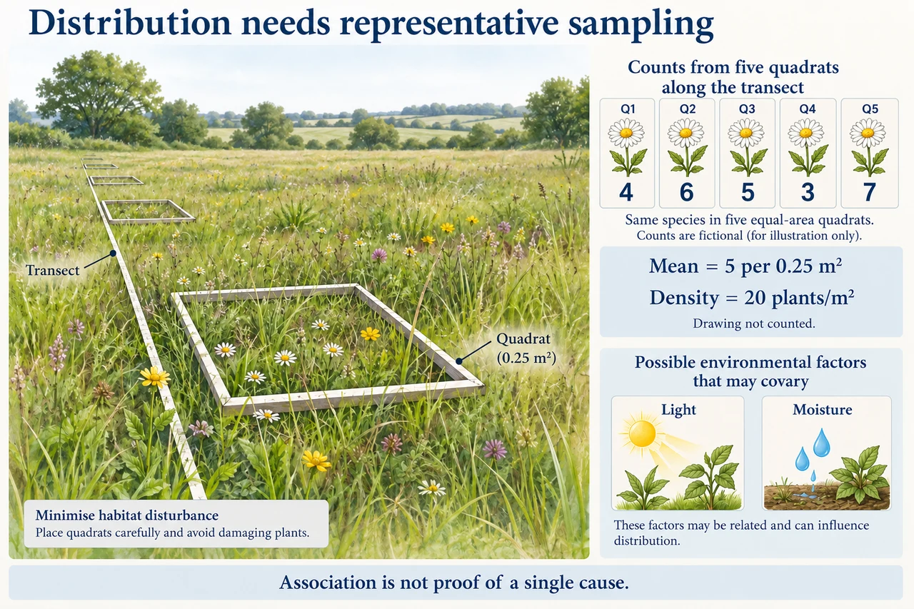
Original myAudience scientific concept illustration; not a photograph or measured specimen. · Original generated project artwork; no source textbook figures reused. Reference links support review, not a copied-art licence.
Relating species distribution to a measured gradient
A distribution study pairs a consistently identified species with a measured environmental factor. A transect is useful for a defined gradient; random quadrats address representative abundance over a sampling frame. Count, percentage cover and presence are different responses, so choose and report the quantity that matches the question.
Comparable quadrat area, observation method and sampling effort support comparisons. Plot the biological response against the measured factor, rather than assuming distance along a transect is the factor itself. Light, moisture, soil and grazing can covary, so an association does not uniquely identify a cause. Repeated independent samples help describe uncertainty but do not repair a biased sampling frame.
Convert mean count per quadrat to density using area; estimates of a total then require a representative habitat area. Zero counts are valid observations. Permissions, site risk assessment and minimal habitat disturbance matter in actual practical work. This lesson prepares analysis for the practical study without claiming that a field investigation or practical endorsement has been completed.
Worked example: Five 0.25 m² quadrats contain 4, 6, 5, 3 and 7 plants. Estimate mean density.
Total count is 25; mean is 25 / 5 = 5 per quadrat.
Divide by quadrat area: 5 / 0.25.
Answer: Estimated mean density is 20 plants/m², subject to representative sampling.
Check your understanding: Does an abundance–light correlation establish light as the only cause?
Answer: No.
Why: Other habitat factors may covary, and the observational design may not isolate one mechanism.