Feedback control: error becomes action, with limits

By How things work · myAudience

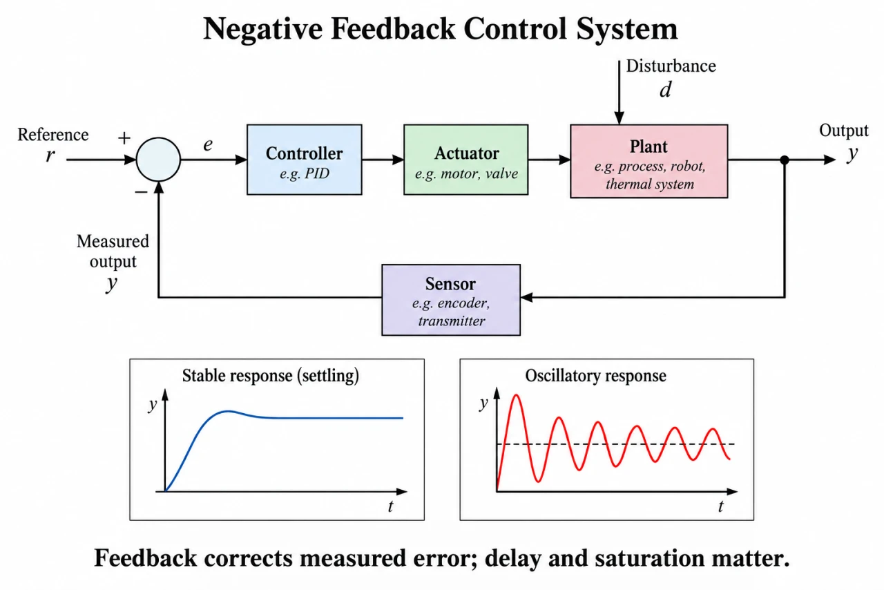
myAudience original imagegen teaching illustration; illustration, not a documentary photograph. · Original generated illustration; scientific and publication acceptance pending independent review.

Feedback control: error becomes action, with limits

A feedback loop measures an output, compares it with a reference and drives an actuator through a controller. For negative feedback e = r − y. The actuator changes the plant, and the sensor closes the loop. A disturbance enters the plant separately from the command; a wrong sensor can make a small measured error coexist with a wrong physical output.

In a deliberately static dimensionless model, y = Gu + d and proportional command u = K(r − y). Substitution gives y = (GK r + d)/(1 + GK). This exposes residual error and disturbance sensitivity, but it says nothing by itself about how a dynamic plant moves toward that value.

Larger positive gain reduces static error in this model. Real delay, inertia and sampling can cause overshoot or oscillation, so a gain that looks attractive algebraically may be unstable dynamically. Integral action accumulates error and can remove some steady offsets if a stable unsaturated solution exists; saturation can instead accumulate excessive command, known as windup.

Efficiency describes energy use and is not the same as tracking accuracy or stability. A controller can track accurately while wasting actuator energy. Sensor calibration, actuator limits, fail states and independent protection must be assessed separately. The diagram shows signal causality, not a safe equipment controller or tuning recipe.

The diagram subtracts measured feedback from reference, passes error through controller and actuator to plant, and feeds sensor output back. A separate disturbance arrow enters the plant. The lower curves are qualitative dynamic responses, not results calculated from the static equations. An oscillating response can decay and remain stable; oscillation alone is not proof of instability.

For discussion, automated control changes who observes faults and who can intervene. Which independent protection, override and accountability should accompany a controller in a consequential setting? Small measured error is not proof of a safe physical state when sensors or actuators can fail.

Image: illustration, not a documentary photograph.

Worked example: Invented normalized static plant G = 2, K = 3, reference r = 1, additive output disturbance d = −0.2. Compute equilibrium output, error and command; verify the plant equation.

GK = 6. y = (6 × 1 − 0.2)/7 = 5.8/7 = 0.828571.

e = 1 − y = 0.171429; u = 3e = 0.514286.

Plant check: 2 × 0.514286 − 0.2 = 0.828572 within rounding. All variables are dimensionless, not volts or temperatures.

Answer: y ≈ 0.828571, e ≈ 0.171429, u ≈ 0.514286 for an unsaturated static model.

Check your understanding: 1: If command clips at u = 0.40, find the consistent output and requested command. 2: If the sensor reads 0.10 above true y without clipping, find true y. Is raising gain proof of stability?

Answer: Clipped output y = 2(0.40) − 0.2 = 0.60; requested u = 3(1 − 0.60) = 1.20, so clipping is self-consistent. With sensor bias, u = 3(1 − y − 0.10); hence 7y = 5.2 and true y = 0.742857. Higher gain is no proof of dynamic stability because dynamics were omitted.

Why: Credit requires testing the assumed saturation regime, locating sensor bias inside the feedback equation and separating static consistency from dynamic stability.