Fibre direction changes what stiffness means

By How things work · myAudience

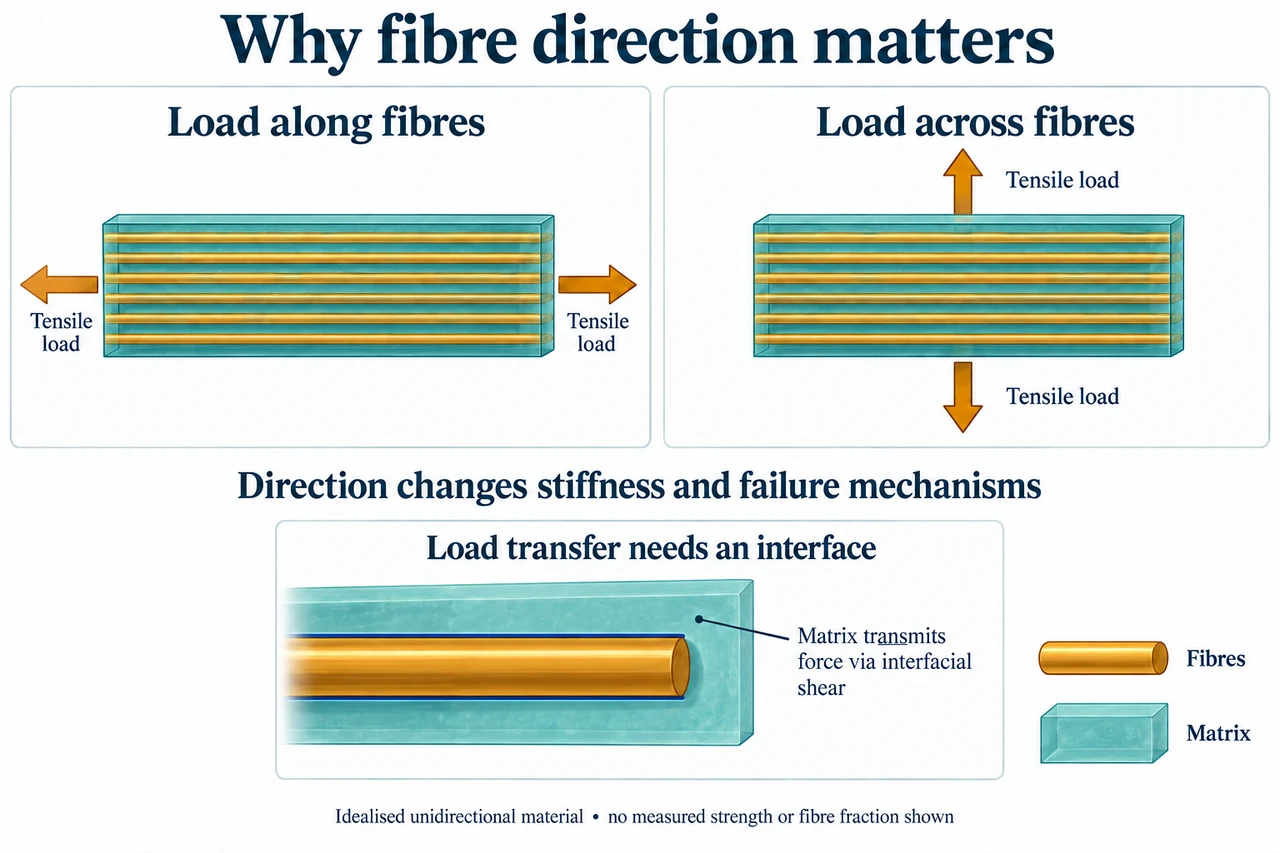
myAudience original rendered teaching illustration. Image: illustration, not a documentary photograph. · Operator-authored generated illustration; scientific model reviewed separately.

Fibre direction changes what stiffness means

A fibre-reinforced composite combines reinforcement with a surrounding matrix. The matrix supports and transfers load to fibres and helps protect them. In the selected unidirectional material, continuous fibres run predominantly in one direction. Its response need not be the same in every direction: this is anisotropy. A claim that a composite is simply stronger needs a direction, a failure criterion and evidence. Stiffness measures resistance to elastic deformation; it is not the stress at which a material fails.

Compare the plate’s two panels. The amber fibres remain horizontal in both; the applied tension changes from horizontal to vertical. That is the intended comparison, rather than secretly rotating the material with the load. The lower inset highlights the interface where the teal matrix and an embedded fibre meet; interfacial shear transfers force, but no measured traction or microscopic concentration is drawn. Poor bonding, voids or damage can defeat a favourable idealised calculation. The illustration does not specify a tested fibre fraction or prove that its two panels have equal strength.

Derive the longitudinal idealisation instead of memorising its answer. Suppose a straight, perfectly bonded, continuous-fibre specimen is loaded along the fibres and both phases remain linear elastic at the same axial strain ε. Their stresses are Ef × ε and Em × ε. For a representative region of equal constituent lengths, area fractions match volume fractions Vf and Vm, with Vf + Vm = 1. Total axial stress is the area-weighted sum, ε(Vf × Ef + Vm × Em). Dividing by ε gives Eparallel = Vf × Ef + Vm × Em. This model assumes effective load transfer and says nothing by itself about a strength limit, short fibres or a multidirectional laminate.

Take original fictional inputs Ef = 120 GPa, Em = 3 GPa and Vf = 0.40, without claiming a particular commercial material. Vm = 0.60, so the longitudinal model gives Eparallel = 0.40 × 120 + 0.60 × 3 = 49.8 GPa. At small strain 0.001, fibre stress is 120 MPa and matrix stress 3 MPa; their weighted mean is 49.8 MPa. In a 100 mm² section the total axial force is 4,980 N because 1 MPa = 1 N/mm². Fibres carry 4,800 N and matrix 180 N in this chosen equal-strain model. These values check force balance, not allowable service loading.

A different serial slab idealisation gives equal stress in two phases and adds their extensions, so 1/Eseries = Vf/Ef + Vm/Em. The same fictional inputs give 1/(0.40/120 + 0.60/3) ≈ 4.918 GPa. Roylance’s MIT 2000 module explicitly warns that this simplified transverse prediction is unreliable for actual fibres because deformation in the matrix is nonuniform. Treat it as an idealised serial comparison or bound under its assumptions, not the tested transverse modulus of our pictured specimen. The large difference explains why changing loading direction deserves new evidence; it does not certify an actual stiffness ratio.

Volume fraction and mass fraction are different. If the fictional fibre and matrix densities are 1,800 and 1,200 kg/m³, a void-free cubic metre with Vf = 0.40 contains 720 kg fibres and 720 kg matrix: fibre mass fraction is 50%, while volume fraction remains 40%. Accidentally inserting 0.50 into the longitudinal volume formula gives 61.5 GPa instead of 49.8 GPa. An engineer would additionally need failure, environment, joint, fatigue and manufacturing evidence. Material savings deserve lifecycle comparison, including difficult separation, repair, production burdens and who bears disposal costs. An attractive lightweight part is not an automatic ethical or environmental improvement.

Image: illustration, not a documentary photograph.

Worked example: Use a fictional void-free, continuous aligned-fibre model with perfect bonding and small equal axial strain: Ef = 120 GPa, Em = 3 GPa, Vf = 0.40. Find longitudinal modulus and forces in a 100 mm² section at strain 0.001. Compute the separate serial-slab comparison and explain its limit.

Vm = 0.60. Eparallel = 0.40 × 120 + 0.60 × 3 = 49.8 GPa.

At strain 0.001, σf = 120 MPa and σm = 3 MPa. Areas 40 and 60 mm² give Ff = 4,800 N and Fm = 180 N, total 4,980 N; effective stress 49.8 MPa agrees with Eparallel × strain.

Eseries = 1/(0.40/120 + 0.60/3) = 300/61 ≈ 4.918 GPa. This serial idealisation is not a reliable measured transverse modulus for an actual fibre geometry.

Answer: Eparallel = 49.8 GPa; phase forces 4,800 N and 180 N balance total 4,980 N. Eseries ≈ 4.918 GPa is only the stated serial model, not a transverse test result or strength rating.

Check your understanding: With fibre/matrix densities 1,800/1,200 kg/m³ and Vf = 0.40, calculate fibre mass fraction. Show the error caused by treating that mass fraction as volume fraction in the longitudinal formula. Can either modulus establish failure strength or justify a weak interface?

Answer: A void-free 1 m³ contains 0.40 × 1800 = 720 kg fibre and 0.60 × 1200 = 720 kg matrix, so fibre mass fraction is 720/1440 = 0.50. Using 0.50 as Vf gives 0.50 × 120 + 0.50 × 3 = 61.5 GPa, 11.7 GPa or about 23.494% above 49.8 GPa. That error is a denominator mistake, not improved material. Modulus is stiffness, not failure strength. A weak interface undermines the perfect-bond assumption and requires a different model and evidence; neither formula repairs it.

Why: Transfer tests the model’s physical assumptions, unit conversions, force balance and the distinction between mass, volume, stiffness and strength. Real composite characterisation requires more than either idealised calculation.