Digital cameras: collecting light is different from amplifying it

By How things work · myAudience

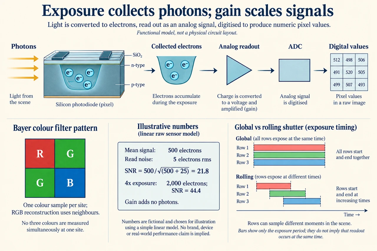
myAudience original generated educational illustration · Original commissioned illustration

Digital cameras: collecting light is different from amplifying it

A digital camera maps arriving light into electrical signals and then numerical samples. In the upper illustration, photons reaching a photosensitive region can produce collected charge; a readout circuit turns that charge into a signal and an analogue-to-digital converter records numbers. The arrow sequence is a functional model, not a transistor layout or a construction drawing. The quantum efficiency used in an example is the fraction of incident photons represented by collected electrons under its stated wavelength and sensor conditions. It is not automatically the same for every colour, device or operating condition.

Exposure time sets the interval over which light is collected. With a steady scene, fixed optical throughput and a linear unsaturated response, a longer interval increases expected collected charge. It can also increase motion blur, and it cannot repair subject detail that moved throughout the interval. Basler’s exposure documentation distinguishes selected and effective exposure times on particular models; those differences warn against assuming that every camera implements an identical timing path. The mechanism is established, while a named camera’s exact timings require its own verified data.

The small colour tile has one red, two green and one blue filter site arranged R-G on the upper row and G-B on the lower row. It is one Bayer arrangement, not a universal sensor design. Each site samples light through its own filter; it does not independently measure complete red, green and blue information at one position. Reconstructing an RGB image estimates missing colour information using neighbours. Edges and fine patterns can challenge that estimation. Basler distinguishes raw Bayer samples from processed RGB output. More numerical output channels do not imply that more independent photons were originally measured.

The numeric card uses a deliberately chosen linear raw-sensor model. Suppose 1,000 incident photons and quantum efficiency 0.50 give a mean signal of 500 collected electrons. Independent Poisson photon arrival contributes a variance of 500 in squared-electron units, while read noise of 5 electrons rms contributes variance 25. Neglect dark signal, quantisation and other noise only for this example. Total noise standard deviation is sqrt(500 + 25), so signal-to-noise ratio is 500 / sqrt(525) = 21.8. The EMVA 1288 linear standard explains this combination of signal-dependent shot noise and independent contributions under its measurement conditions; the simplified equation is not a complete model of processed phone photographs.

Four times the exposure produces a mean of 2,000 electrons under unchanged steady illumination and unsaturated linear operation. With the same 5-electron rms read noise, SNR becomes 2,000 / sqrt(2,025) = 44.4. The signal grew fourfold, but the SNR roughly doubled because shot-noise standard deviation also grows with the square root of signal. In the shot-noise-dominated limit, SNR tends to sqrt(N), so four times N gives twice the SNR. In a read-noise-dominated regime the scaling can differ; do not apply a single scaling rule without inspecting the terms.

Gain scales a signal; it adds no incident photons. Basler distinguishes analogue gain before conversion from digital multiplication after conversion, with model-dependent availability. An ideal scaling that multiplies signal and existing noise equally leaves their ratio unchanged, although gain can affect how quantisation and downstream noise enter a real measurement. It can also reduce available headroom. If a fictional collected-charge limit is 2,400 electrons, a pixel starting at 800 electrons would be expected to reach 3,200 after fourfold exposure and therefore clip. A different pixel starting at 500 reaches 2,000 and can remain unsaturated. Amplifying or editing the clipped output cannot recover the original unknown excess signal.

The two timing grids compare exposure intervals, not complete readout electronics. Global exposure bars begin and end together; rolling exposure bars are offset from row to row. A moving edge can then be sampled at different positions in different rows, producing distortion. Global exposure does not mean all pixel values are read out instantaneously; Basler describes row-by-row readout after common exposure on its global-shutter examples. Noise and timing trade-offs are sensor-specific, so this picture is not a universal ranking of camera quality.

Better imaging can support science, accessibility and documentation, but capture also affects privacy and consent. A technically clearer image is not permission to identify or monitor people. Decide which detail a task truly needs, whether bystanders can consent and how long the data should remain. Explain processing or generated content when it changes the evidential meaning of an image. Image: illustration, not a documentary photograph. Its selected values and colour grid teach mechanisms rather than report a device benchmark.

Worked example: In a fictional linear raw pixel, 800 incident photons and quantum efficiency 0.50 give the mean collected charge. Read noise is 4 electrons rms. Calculate SNR, then repeat for twice the exposure. Assume steady illumination, no clipping, negligible dark and quantisation terms.

Mean charge = 800 × 0.50 = 400 electrons; read-noise variance = 4² = 16 electrons².

SNR = 400 / sqrt(400 + 16) = 19.61.

Twice the exposure gives 800 electrons; SNR = 800 / sqrt(800 + 16) = 28.01. The ratio is about 1.43, not 2.

Answer: Approximately 19.6 and 28.0; the signal doubles while the combined noise also changes.

Check your understanding: A pixel at 900 electrons has a fictional 2,400-electron charge limit. Will three times the exposure remain linear? Will doubling a digital sample recover any clipping? Separately, two rolling-shutter rows begin 2 ms apart; an edge moves across the image at 300 pixels/s. Find the difference in edge position and name the missing information for a full image-distortion prediction.

Answer: The expected charge is 2,700 electrons, exceeding the stipulated limit, so the unqualified linear prediction fails. Digital gain cannot recover the clipped excess or add photons. The row-start difference corresponds to 300 × 0.002 = 0.6 pixel of motion for the stipulated constant image velocity. Full distortion also needs all row timings, direction and motion, exposure duration and scene geometry; this two-row estimate is not a complete camera model.

Why: Use the declared model and explain which physical or protocol assumptions prevent an unrestricted real-device prediction.