Irrigation: account for water in the root zone

By How things work · myAudience

myAudience original generated educational illustration · Original commissioned illustration

Irrigation: account for water in the root zone

Irrigation supplies water when rainfall and stored soil water do not meet the relevant crop demand. Pouring water onto a field is not the same as retaining it where roots can use it. FAO’s established water-balance framework distinguishes rain, net infiltration, evapotranspiration, runoff and drainage; its older models are explanatory references here, not a current local irrigation prescription. Root depth, soil properties, crop stage, weather, salinity and measurement quality all affect an actual decision. This lesson builds a declared water balance before judging whether a larger delivered volume is useful.

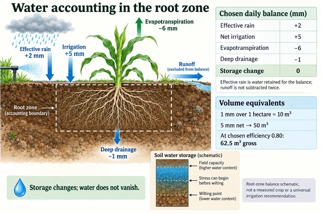
Read the dashed root-zone boundary on the plate. Rain and irrigation enter from above; evapotranspiration leaves through evaporation and plant transpiration; drainage crosses the bottom of the zone; runoff leaves at the surface. The numerical table uses effective rain after the relevant runoff exclusion, so runoff is not subtracted a second time. Its chosen daily inputs are 2 mm of effective rain and 5 mm of net irrigation, while 6 mm leaves as evapotranspiration and 1 mm as deep drainage. Their balance is zero storage change. The drawing does not mean a real root zone is a rigid tank or water is uniformly distributed through it.

Use one explicit sign convention: ΔS = Pe + I + C − ET − D, where ΔS is change in stored root-zone water, Pe is effective rain included in this balance, I is net infiltrated irrigation, C is capillary contribution from below, ET is actual evapotranspiration and D is drainage beyond the zone. All are depths over the same area and time interval. Choose C = 0 for the plate. A positive ΔS adds storage; a negative value depletes it. FAO also writes balances in terms of depletion, whose sign changes relative to storage. Mixing the two conventions without naming them can reverse the conclusion.

Millimetres are a convenient depth equivalent, not tiny bottles of water. One hectare is 10,000 m², so 1 mm = 0.001 m over that area is 10 m³. The plate’s 5 mm net irrigation therefore represents 50 m³ entering the chosen root-zone boundary. If a declared overall delivery efficiency is 0.80, gross supply for that net quantity is 50 / 0.80 = 62.5 m³. The remaining 12.5 m³ lies outside the net quantity in this simplified model; it is not automatically all evaporated or permanently lost to the wider basin. Efficiency must name its boundary and time period.

Soil water also has availability limits. Field capacity and wilting point are reference conditions, not universal percentages for all soils. As a chosen uniform-root-zone illustration, volumetric water contents of 0.30 and 0.15 m³/m³ across a 0.60 m root depth imply (0.30 − 0.15) × 0.60 = 0.090 m, or 90 mm, between those reference contents. Plants can become stressed before all of that interval is depleted. The storage strip in the image marks that qualitative distinction without supplying a crop-specific threshold. A total volume alone cannot tell whether all roots can access it, and a uniform-depth calculation omits spatial variation. The small blue storage strip is a symbolic accounting reference, not a literal perched water table or measured saturated soil layer.

Test a proposed schedule by transferring the balance, not by copying a pictured number. Suppose starting storage relative to a chosen reference is 40 mm, effective rain is 1 mm, net irrigation is 4 mm, ET is 7 mm and drainage is zero. Then ΔS = −2 mm and the final storage is 38 mm under the model. Without irrigation it would be 34 mm, not zero. Repeating a fixed ET value indefinitely would eventually break the model because water stress can alter actual transpiration; rain, root growth and soil conditions may also change. A one-day accounting check is not a season-long yield prediction.

Water-efficient equipment and basin-wide conservation are related but not identical. Reduced runoff or drainage may reduce withdrawals at one farm, yet those flows may formerly have supplied downstream users or groundwater recharge; expansion of irrigated area can change total demand. Evaluate groundwater, ecosystem needs, livelihoods, pumping energy and access alongside field delivery efficiency. Salinity management and nutrient leaching can create additional constraints absent from the table. Avoid presenting a single efficiency number as a moral ranking of farmers whose soils, water rights and resources differ; explain the assumptions and who is affected.

Image: illustration, not a documentary photograph. The root-zone arrows and original chosen numbers teach accounting; the storage strip is qualitative and provides no irrigation schedule, crop threshold or yield guarantee.

Worked example: For a fictional 2-hectare field, net irrigation is 6 mm in one day. Effective rain is 3 mm, ET is 7 mm, drainage is 1 mm and capillary rise is zero. Find storage change, net irrigation volume and gross supply at a chosen efficiency of 0.75.

Storage change = 3 + 6 + 0 − 7 − 1 = +1 mm.

One millimetre over 2 hectares is 0.001 × 20,000 = 20 m³; net irrigation = 6 × 20 = 120 m³.

Gross supply = 120 / 0.75 = 160 m³. The 40 m³ outside the net quantity is not automatically consumptive loss from the entire basin.

Answer: Storage increases 1 mm in the model; 120 m³ net requires 160 m³ gross at the stated efficiency.

Check your understanding: A report records 5 mm total rain and 2 mm runoff, then calls effective rain 3 mm. Net irrigation is 4 mm, ET is 6 mm and drainage 1 mm. Someone subtracts runoff again and obtains −2 mm. Correct the balance. For chosen θFC = 0.28, θWP = 0.12 and root depth 0.50 m, calculate the reference available-water interval; does it all remain readily available without stress?

Answer: Use effective rain only once: ΔS = 3 + 4 − 6 − 1 = 0 mm. Subtracting the 2 mm runoff again double-counts it. The chosen reference interval is (0.28 − 0.12) × 0.50 = 0.080 m = 80 mm. That is not a guarantee of stress-free extraction of all 80 mm; the onset of stress and accessibility depend on crop and soil conditions.

Why: State the system boundary, trace the mechanism, use consistent units and justify what the simplified calculation cannot establish.