X-ray and CT: a projection is not a complete picture

By How things work · myAudience

myAudience original generated educational illustration · Original commissioned illustration

X-ray and CT: a projection is not a complete picture

X-ray imaging measures radiation that reaches a detector after interacting with an object. Some photons are absorbed, some scatter into different directions and some pass through. A conventional radiograph combines information along each ray path into a projection: structures at different depths can overlap. Computed tomography acquires projections from multiple directions and uses a mathematical reconstruction to estimate a spatial distribution of attenuation. The useful distinction is not that CT sees with a different kind of light, but that it gathers additional geometrical evidence and solves an inverse problem. This mechanism is established; a reconstruction still depends on sampling, signal quality and assumptions.

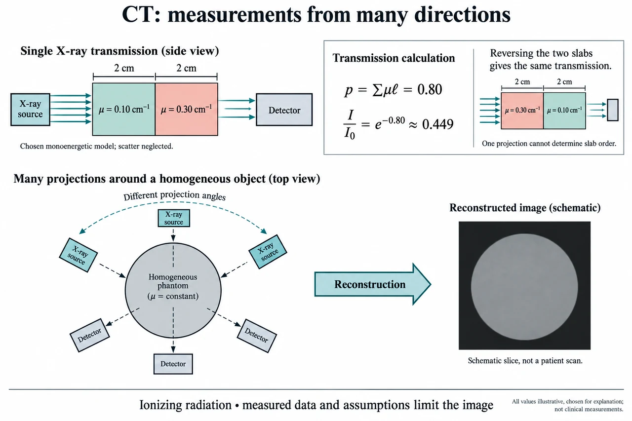
The illustration first isolates a deliberately simple ray. Two uniform slabs, each 2 cm thick, lie between a source and a detector. Their chosen attenuation coefficients are 0.10 cm⁻¹ and 0.30 cm⁻¹. Here the beam has one energy, the coefficients are constant within each slab, and scattered radiation reaching the detector is neglected. These assumptions allow primary transmitted intensity to be written as I = I₀ exp(−Σμℓ), where μ is attenuation coefficient and ℓ is path length. Each μℓ is dimensionless: cm⁻¹ multiplied by cm. The drawing is an original conceptual phantom, not tissue measurements, a patient scan or a description of an actual clinical spectrum.

For this selected ray, the exponent’s positive path sum is p = 0.10 × 2 + 0.30 × 2 = 0.80. Transmission I/I₀ = exp(−0.80) is approximately 0.449, so about 44.9% of the incident primary intensity remains in the ideal model. Reversing the order of the two slabs leaves the same sum and therefore the same transmitted fraction. This is a demanding limitation rather than a small detail: one projection cannot identify which slab came first along that path. Applying −ln to a correctly normalised transmitted fraction recovers a line-integral estimate, not the separate local coefficients or the material order. Extra views constrain the spatial arrangement.

The lower illustration shows a source and an opposite detector at different positions around a generic phantom. It represents successive projection geometries, not a scanner that must contain several simultaneously operating sources. Combining many rays and angles allows reconstruction of slices and, with appropriate acquisition, volumetric information. The reconstructed image is not a direct optical photograph inside the body. Finite angular sampling, motion, noise and the algorithm used can all influence it. Real X-ray beams contain a range of energies; attenuation changes with energy and preferential removal of lower-energy photons can produce beam-hardening effects. Scatter also complicates the simple exponential route. The chosen slab calculation is a bounded explanation of primary transmission, not a complete CT simulator.

Consider what happens when the source intensity changes. If I₀ is 1,000 arbitrary signal units, the chosen slabs produce approximately 449 units at the detector. If I₀ doubles and all other ideal assumptions hold, the detector receives approximately 899 units, while the normalised fraction remains 0.449 and p remains 0.80. That invariance does not mean clinical exposure is irrelevant. With ideal independent photon-count fluctuations, relative counting uncertainty scales approximately as 1/√N, so more counts can improve statistical precision. Detector response, scatter, motion and model error still matter. A signal unit or a transmitted photon count is not an absorbed-dose measurement and cannot determine risk by itself.

Image samples and reliable detail must also be distinguished. Dividing a 240 mm field into 240 samples gives a 1 mm sampling interval; using 480 samples gives 0.5 mm. Doubling the number of displayed samples does not prove that the system resolves features half as large. The acquisition geometry, detector response, reconstruction, noise and movement determine what information survives. Interpolation can make a smooth image without creating new measured evidence. New reconstruction or AI methods therefore need validation for their intended use, with attention to errors and failure conditions rather than judging only visual attractiveness. The source pages used here establish mechanism and safety principles, not a ranking of the latest scanners or a guarantee about any particular algorithm.

X-rays are ionizing radiation, unlike the RF used in MRI. FDA explains that medical use balances the information needed with radiation-related risks, and that appropriate examination and image quality are part of that judgement. Neither this lesson nor its fictional attenuation coefficients establishes a dose, a diagnostic threshold or a suitable examination for a person. Contrast agents and clinical protocols introduce additional considerations requiring professional assessment. Ethics includes justified use, equitable access, honest communication of uncertainty, and protection of identifiable imaging data. A reconstructed finding must be interpreted in clinical context; a plausible-looking image is not automatic evidence of disease or its absence.

Image: illustration, not a documentary photograph. The upper beam route explains a monoenergetic, scatter-neglected primary-transmission model and why slab order cannot be inferred from one ray. The lower angular views explain the added information used in reconstruction; the invented grayscale slice is not a scan or a clinical result. This lesson does not cover every CT architecture, dosimetry method or reconstruction algorithm.

Worked example: A chosen monoenergetic beam crosses 3 cm of a uniform material with μ = 0.20 cm⁻¹ and negligible detected scatter. Calculate p and transmission. For I₀ = 800 arbitrary units, calculate I. Double I₀ without changing the object and compare normalised transmission. Separately compare sampling intervals for a 240 mm field represented by 240 or 480 samples.

p = μℓ = 0.20 × 3 = 0.60, with cm⁻¹ and cm cancelling. I/I₀ = exp(−0.60) ≈ 0.5488.

I = 800 × 0.5488 ≈ 439 arbitrary units. At I₀ = 1,600, I ≈ 878 units. The normalised fraction and p remain unchanged in the ideal model.

The intervals are 240/240 = 1 mm and 240/480 = 0.5 mm. This is a sampling calculation, not proof of actual spatial resolution, absorbed dose or diagnostic accuracy.

Answer: The ideal path sum is 0.60 and transmission approximately 0.5488; doubling the incident intensity doubles the detector signal without changing the normalised fraction. Sampling intervals are 1 mm and 0.5 mm, with acquisition limits still separate.

Check your understanding: The plate’s two equal-thickness slabs are reversed. Does the transmitted fraction change, and can one ray locate their order? If an ideal detector counts 400 independent photons in one acquisition and 1,600 in another, compare approximate relative counting uncertainty. Does the improvement establish clinical safety or eliminate reconstruction artifacts?

Answer: The path sum remains 0.80 and transmission remains approximately 0.449; one ray cannot identify the slab order. The ideal relative counting uncertainties are 1/√400 = 5% and 1/√1,600 = 2.5%. This particular statistical uncertainty halves, but other uncertainties and exposure considerations remain. It does not establish dose, safe operation, clinical accuracy or elimination of artifacts.

Why: Track the measured signal, model assumptions, units and inference separately; explain why numerical precision does not establish clinical accuracy.