MRI: resonance, encoding and the limits of an image

By How things work · myAudience

myAudience original generated educational illustration · Original commissioned illustration

MRI: resonance, encoding and the limits of an image

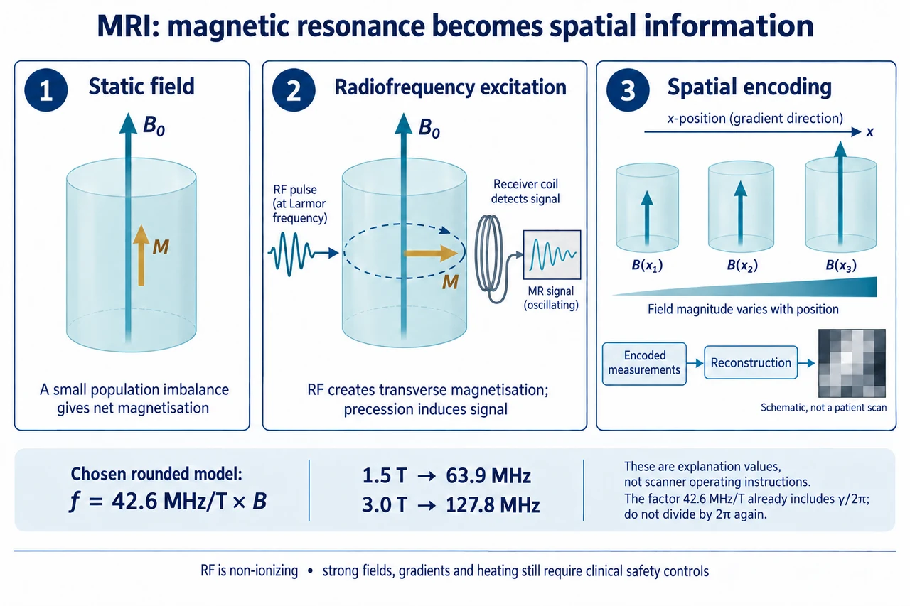
MRI uses magnetic fields and radiofrequency signals to obtain information about a sample, commonly through hydrogen nuclei in biological tissue. It does not use the ionizing X-rays used by CT. The hydrogen nucleus has a magnetic moment and quantum spin; the textbook arrows are representations of magnetisation, not miniature mechanical balls rotating inside the body. In a static magnetic field there is a small population imbalance between allowed spin states, producing a net longitudinal magnetisation. It is incorrect to say every proton points in the same direction. The plate deliberately shows one net magnetisation vector, rather than identical arrows for every nucleus.

A suitable RF excitation changes the net magnetisation so that a transverse component can precess around the static field direction. The time-varying transverse magnetisation induces an oscillating electrical signal in a receiving coil. This signal is evidence that must be encoded and processed; it is not an anatomical photograph. The second panel shows the RF input and the transverse vector’s precession around the vertical field axis. It does not supply a pulse prescription, scanner setup or coil construction plan. Microscopic ensembles and quantum transitions are more complex than the useful net-vector model, but that model distinguishes equilibrium magnetisation, excitation and detection without claiming every proton behaves identically.

In the simple proton resonance model, f = (γ/2π)B. NIST’s 2022 CODATA table gives the proton factor in MHz/T as approximately 42.5775; this lesson deliberately rounds it to 42.6 MHz/T for arithmetic. Multiplying that rounded factor by 1.5 T gives 63.9 MHz, and multiplying by 3.0 T gives 127.8 MHz. Because the factor is already expressed as cycles per second per tesla, dividing by 2π again would be wrong. Local chemical environment and shielding modify precise resonance conditions, and the two displayed values are explanation models rather than clinical operating instructions or proof that one field strength produces a better diagnosis.

A receiver signal alone does not say where every contribution originated. Spatial encoding uses controlled magnetic-field gradients: the field component along the main field varies with position, so positions can acquire different frequencies or accumulated phases. The plate’s third panel therefore shows parallel upward arrows with different lengths, not magnetic vectors turning sideways with x-position. Slice selection and frequency and phase encoding provide complementary spatial information. Encoded measurements are collected in a mathematical data space commonly called k-space; reconstruction, often using Fourier methods, relates this information to a spatial image. K-space is not already a miniature anatomical picture, and its completeness and quality affect the result.

Several timing processes influence contrast. Longitudinal recovery is described by T1, while loss of coherent transverse magnetisation in an ideal model is described by T2. Field inhomogeneity contributes additional dephasing, commonly reflected in T2*, so one observed decay should not automatically be labelled pure T2. Relaxation times depend on the tissue and measurement conditions. They are not the amount of energy in a single spinning nucleus or a universal healthy-versus-unhealthy threshold. Contrast also depends on acquisition choices and processing; the image’s brightness cannot be read as a simple direct count of hydrogen or as an automatic diagnosis. This mechanism lesson does not prescribe a clinical sequence.

Sampling provides another useful quantitative boundary. With a 240 mm field of view across 120 samples, the nominal in-plane spacing is 2 mm. Across 240 samples, it is 1 mm. If an illustrative slice thickness is 4 mm, the corresponding nominal voxel volumes are 2 × 2 × 4 = 16 mm³ and 1 × 1 × 4 = 4 mm³. Finer samples do not guarantee that real features this small can be resolved: acquisition, noise, field imperfections, motion and reconstruction affect reliable detail. A smaller voxel can reduce the signal available from each element under otherwise comparable conditions; there is no cost-free promise that increasing matrix size makes every image better. These are geometric chosen models, not specifications for a scanner or a scan.

Non-ionizing does not mean harmless. FDA describes strong-field projectile hazards, RF heating, gradient-related effects and acoustic noise, along with the importance of implant and accessory safety. MR Safe and MR Conditional labels differ: a conditional device is acceptable only under its identified conditions, not simply because it is made partly of metal or has been scanned before. Unknown status cannot be assumed compatible. Clinical screening, patient communication, professional equipment controls and interpretation belong to qualified practice. Equity also includes access, comfort, accommodations and valid evidence for the intended population; a noisy or incomplete acquisition should be described honestly rather than cosmetically replaced with a reassuring reconstruction.

Image: illustration, not a documentary photograph. The three panels connect net magnetisation, RF excitation and spatial encoding; the generic grayscale block is not a patient image. All vectors are bounded conceptual representations, the resonance values use a deliberately rounded constant, and no anatomical or diagnostic claim is implied. Full pulse-sequence design, quantitative relaxation measurement, contrast-agent decisions and clinical safety clearance remain outside this lesson.

Worked example: Using the deliberately rounded proton factor 42.6 MHz/T, find the resonance frequency for a chosen field of 2.0 T. For an unrelated geometric example, use a 256 mm field represented by 128 and 256 samples, with a chosen 3 mm slice thickness. Calculate spacing and nominal voxel volumes, then explain why smaller pixels alone do not prove better diagnostic accuracy.

f = 42.6 × 2.0 = 85.2 MHz in the chosen rounded resonance model; no additional division by 2π is required.

The spacings are 256/128 = 2 mm and 256/256 = 1 mm. Nominal voxel volumes are 2 × 2 × 3 = 12 mm³ and 1 × 1 × 3 = 3 mm³.

The nominal volume falls by a factor of four. Reliable resolution and accuracy still depend on acquisition, signal, motion, encoding and reconstruction; these geometric calculations provide no clinical settings or diagnostic guarantee.

Answer: The chosen model gives 85.2 MHz. Sampling spacings are 2 mm and 1 mm, and nominal voxel volumes are 12 mm³ and 3 mm³, separate from demonstrated resolution and clinical performance.

Check your understanding: A learner says every proton aligns with the magnet, a gradient turns the field sideways, and MRI uses no radiation so all implants are safe. Correct these claims. Would a nominal 1 mm pixel prove that two objects 1 mm apart are reliably distinguishable?

Answer: A small spin-population imbalance produces net magnetisation; not every proton is identical or aligned. Spatial gradients vary the main-field component with position, rather than requiring it to point sideways. MRI uses non-ionizing RF, not ionizing X-rays, but field, heating, noise and implant hazards remain; MR Conditional conditions and professional screening matter. A pixel is a sample, not a demonstrated resolution guarantee, so reliable distinction requires additional evidence.

Why: Track the measured signal, model assumptions, units and inference separately; explain why numerical precision does not establish clinical accuracy.