ECG: a measured voltage is evidence, not a complete heart assessment

By How things work · myAudience

myAudience original generated educational illustration · Original commissioned illustration

ECG: a measured voltage is evidence, not a complete heart assessment

An electrocardiogram records electrical activity associated with the heart. It is not an ultrasound picture, a blood-pressure measurement or a direct measurement of pumping strength. Cardiac cells change their membrane potentials as electrical activity propagates through a specialised conducting system and the muscle. Surface electrodes detect the combined electrical effect through the body, rather than recording one isolated cell’s membrane voltage. NIH describes the sinoatrial node, atrial propagation and atrioventricular delay as parts of the heartbeat’s conduction sequence. Electrical activation and subsequent mechanical contraction are connected, but they are distinct events; a recognisable electrical signal does not by itself prove effective circulation.

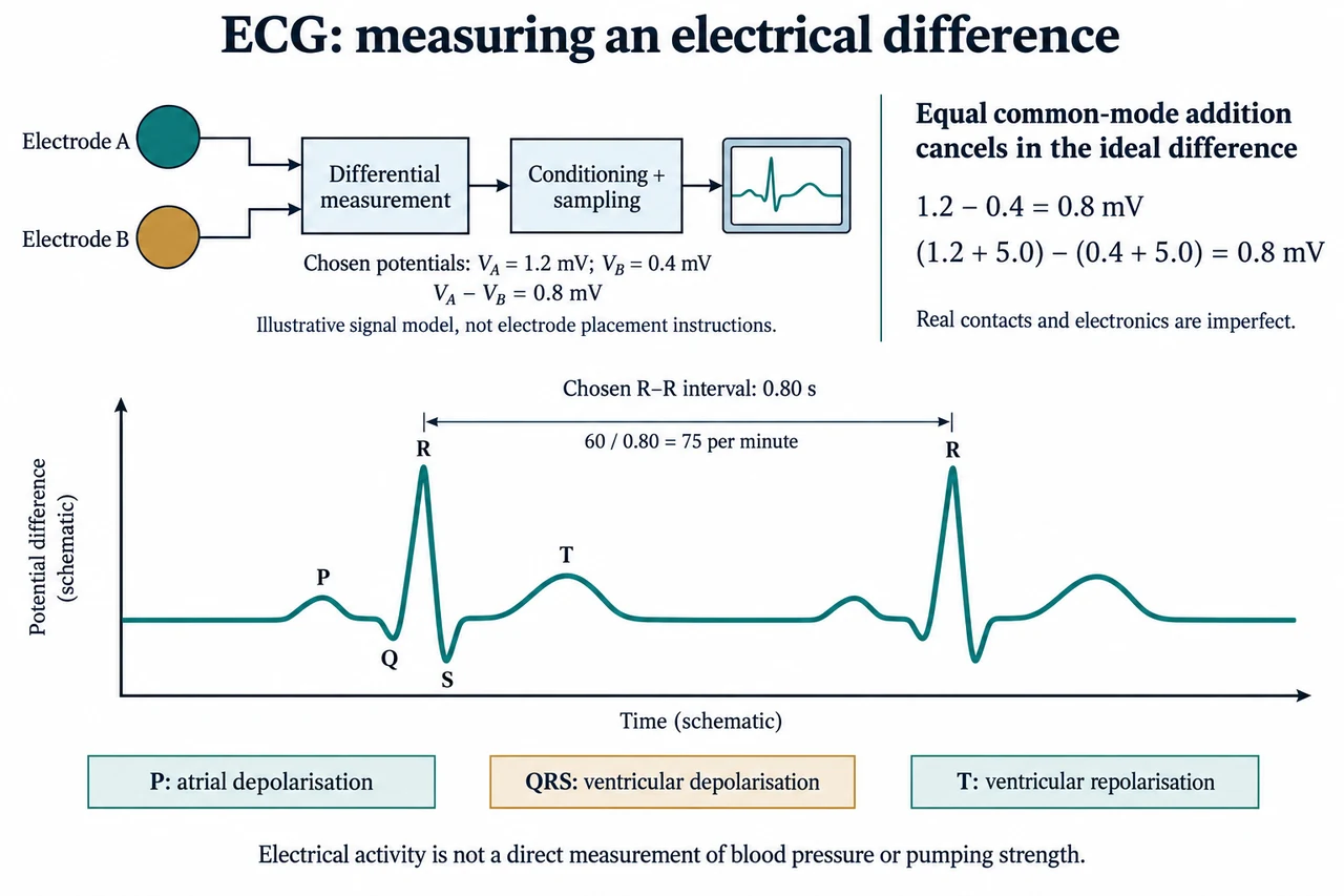
The upper illustration begins with two abstract electrodes, A and B, with fictional potentials referred to the same chosen reference. Their values are 1.2 mV and 0.4 mV, so the ideal measured difference is 0.8 mV. A lead is a specified electrical view, not necessarily a separate electrode or a literal cable. A standard twelve-lead ECG obtains its views using ten electrodes; one wearable channel is not twelve independent views of the heart. The abstract circles are intentionally not a placement guide. The voltage pattern depends on the view, the distributed cardiac activity, the body’s conducting properties and the electrode interface, not just the strength of one contraction.

Subtracting the two inputs illustrates common-mode rejection. If the same chosen 5.0 mV disturbance is added to both, (1.2 + 5.0) − (0.4 + 5.0) still equals 0.8 mV. This cancellation holds for the ideal difference under matched conditions. If the additions instead become 5.0 mV and 4.9 mV, the difference is 0.9 mV: the extra 0.1 mV survives as a differential error. Relative to the original 0.8 mV signal, that is 12.5% in this selected example. Real electrode impedances and electronics can turn common disturbances into unequal input effects. The exercise therefore explains why a mathematical subtraction alone is not proof of a noise-free physiological measurement.

A practical acquisition system must preserve a small time-varying signal while handling electrode offsets, contact changes, motion and environmental interference. Conditioning and sampling turn the analogue measurement into data for display and analysis. Filtering can suppress unwanted components, but it can also alter timing or waveform detail; visual smoothness is not a sufficient validation criterion. The manufacturer sources consulted describe input impedance, electrode mismatch, differential offsets and anti-aliasing as engineering concerns, not a universal guarantee of clinical performance. This lesson gives no circuit, electrode connection, patient-drive instruction or device operating settings. Electrical safety and intended-use validation require much more than obtaining a plausible trace.

In the plate’s schematic P–QRS–T pattern, P represents atrial depolarisation, QRS represents ventricular depolarisation and T represents ventricular repolarisation. The atrial repolarisation contribution is commonly obscured by ventricular activity. These named electrical features are not literal pressures or valve sounds, and an upward peak is not a quantity of blood pushed out. Different leads can show different polarity and shapes; the selected positive P and T with a tall R are an explanatory pattern, not the only valid morphology. Actual diagnostic interpretation includes relationships, intervals, clinical context and more than one channel when appropriate. No disease is assigned to this invented drawing.

Equivalent neighbouring R peaks in the image have a chosen separation of 0.80 s. In a clean regularly repeating model, the repetition frequency is 1/0.80 = 1.25 Hz and the number of repetitions per minute is 60/0.80 = 75. The uncalibrated horizontal axis is labelled schematic, so the bracket supplies the fictional time rather than claiming a measured paper speed. At an illustrative sampling rate of 250 samples/s, the nominal sample interval is 4 ms. An interval of 200 sample spacings corresponds to 0.80 s; it is not an interval of 200 stored points including both endpoints, which would span 199 spacings. Timing depends on the selected feature and sampling assumptions, while noise and imperfect peak detection add further uncertainty.

An average rate can conceal irregular timing. For three chosen successive intervals of 0.60 s, 1.00 s and 0.80 s, the mean interval is 0.80 s and three intervals occupy 2.40 s, giving 75 repetitions/minute over that elapsed span. Averaging the separate instantaneous rates, 100, 60 and 75, instead gives about 78.3 and is a different statistic. Neither number diagnoses the cause of the variability. Clinical interpretation and follow-up belong to qualified professionals, as the NHS explains. Ethical design should protect sensitive recordings, make uncertain or unusable measurements visible and avoid treating access to a watch as a substitute for appropriate healthcare. Evidence needs to reflect the intended users and recording conditions, rather than only a clean laboratory trace.

Image: illustration, not a documentary photograph. The top boxes teach an ideal differential measurement with chosen voltages; the lower trace is original and uncalibrated except for its explicitly chosen R–R interval. It is not a patient record, lead-placement guide, diagnostic threshold, device construction plan or full ECG interpretation course. All waveform names and quantitative examples are explained here so the illustration does not replace the reasoning.

Worked example: Use fictional electrode potentials A = 2.0 mV and B = 0.7 mV. Compute their difference, then add an equal 3.0 mV disturbance to each. If the additions become 3.0 and 2.8 mV, calculate the residual error. For an unrelated clean model sampled at 250 samples/s, two equivalent peaks are 225 sample spacings apart: calculate interval and repetitions per minute.

The original difference is 2.0 − 0.7 = 1.3 mV. Equal additions give (2.0 + 3.0) − (0.7 + 3.0) = 1.3 mV in the ideal model.

Unequal additions give 5.0 − 3.5 = 1.5 mV, leaving an added 0.2 mV error. The mismatch survives differential subtraction.

The interval is 225/250 = 0.90 s, so the clean repetition rate is 60/0.90 ≈ 66.7 per minute. No clinical category follows from these invented values.

Answer: The ideal difference is 1.3 mV and is unchanged by equal disturbance; unequal disturbance leaves 0.2 mV added error. The separate timing model gives 0.90 s and approximately 66.7 repetitions/minute.

Check your understanding: Does a tall R prove strong pumping or adequate circulation? Why are twelve leads not twelve electrodes? Compare the elapsed-span rate for intervals 0.60/1.00/0.80 s with the mean of their separate reciprocal rates, and explain why a smooth wearable trace is not a complete cardiac assessment.

Answer: R is part of a measured electrical view, not direct mechanical output or blood flow. A standard twelve-lead view set uses ten electrodes; lead and electrode are different concepts. Three intervals occupy 2.40 s, so the elapsed-span rate is 3 × 60 / 2.40 = 75/min; the mean of 100, 60 and 75 is 78.3/min and represents another statistic. Different views, signal quality, timing patterns and clinical context matter; smoothness alone does not establish complete assessment.

Why: Explain the signal or transport boundary, identify model assumptions, calculate with units and distinguish a chosen model from clinical interpretation.