Traffic signals: arrivals, service and the cost of shared time

By How things work · myAudience

myAudience original generated educational illustration · Original commissioned illustration

Traffic signals: arrivals, service and the cost of shared time

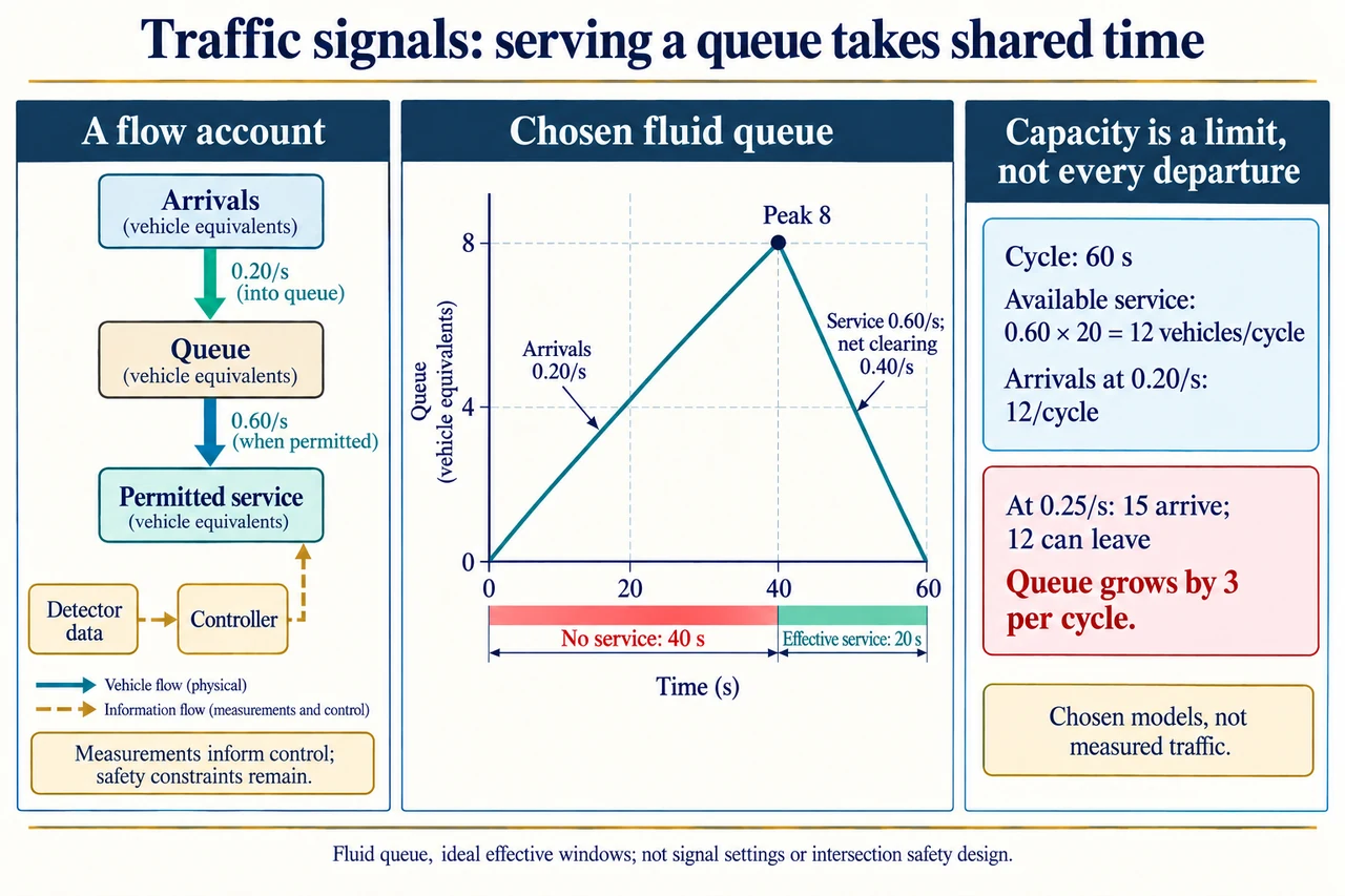
A traffic signal allocates access through a shared space among movements that cannot all be served together. Its controller responds to timing rules and, in some systems, detections or measured demand. A useful explanation separates physical arrivals and departures from information used to choose service. The image's left panel uses solid arrows for the flow into a queue and onward through permitted service, while dashed arrows connect detector data to a controller. More information does not remove the need for conflict prevention, pedestrian access or properly engineered safety constraints. This article uses an abstract queue, not a road intersection layout or a set of signal settings to install.

The queue follows conservation: Q(t + Δt) = Q(t) + arrivals − departures, with Q never negative. A detector's observed departure count is not automatically the number who wanted to arrive. An upstream blockage can keep people from reaching the queue, and a downstream blockage can stop an apparently permitted movement from discharging. The FHWA teaching manual makes this demand-versus-volume distinction. The image's rate values are chosen fluid-model equivalents in vehicles per second, allowing a smooth line instead of the individual jumps of actual cars. The graph assumes a continuously available downstream destination, fixed arrivals and ideal service; it is not a measured traffic trace.

In the central chosen account, a 60 s cycle consists of 40 s with no service followed by 20 s of effective service. Starting with Q = 0, arrivals at 0.20 vehicle-equivalents per second create a queue of 0.20 × 40 = 8 at the start of service. During service, departures can occur at 0.60 per second while arrivals continue at 0.20, so the queue falls at the net rate 0.40 per second. Clearing 8 therefore takes 20 s, returning to zero at the cycle's end. The straight graph rises from(0,0) to(40,8) and falls to(60,0). The descending slope is not 0.60 because that would forget continuing arrivals; net change is arrivals minus departures. The plotted geometry is illustrative; use the stated values rather than pixel distances for calculations.

Available service is 0.60 × 20 = 12 vehicles per cycle, or 12/60 = 0.20 per second averaged across the cycle. The original arrivals also total 12, leaving no capacity margin in this exact deterministic account. If arrivals instead average 0.25 per second,15 arrive during a cycle while at most 12 can be served, so a persistently busy queue grows by 3 per cycle. Starting empty, it grows to 10 during the first no-service interval, then falls by 7 during service, leaving 3. The next cycle leaves 6 if assumptions persist. A controller cannot serve 15 through a window physically capable of only 12 merely by predicting arrivals better. At exactly matched average demand, random variation can also leave residual queues; exact repeated clearing is a fragile feature of this idealised example.

The area under the queue graph adds a different outcome from peak length. For the original triangle, it is½ × 40 × 8 + ½ × 20 × 8 = 240 vehicle-equivalent seconds per cycle. Each waiting vehicle contributes one vehicle-second for each second in the queue, so this area measures accumulated queue waiting. Dividing by 60 gives an average queue of 4 vehicle equivalents. Dividing by the 12 arrivals served in that repeating cycle gives mean queue wait 20 s, consistent with L = λW when the periodic steady accounting boundary matches. This is queue waiting only: it excludes travel through the intersection, starting response, deceleration and other real delay. For a growing queue, a finite-cycle average is not a stationary long-run waiting-time prediction.

Effective service time is a modelling window, not necessarily the duration of a displayed green light. Real approaches have start-up response, clearance intervals, different users and conflict rules. Here these effects are excluded or already absorbed into the chosen effective 20 s; the diagram's red and green bands show abstract unavailable/available service, not permissions for a real road user. Adding time to this movement within a fixed cycle takes shared time from another use, unless some other term changes. A local improvement can therefore delay a side street, a pedestrian or a bus, or send a queue into another junction. Whole-network performance cannot be concluded from one queue's lower peak or an isolated vehicle throughput total.

Established adaptive control uses measurements to adjust service choices as conditions change. FHWA's April 2023 programme handbook distinguishes selecting among predefined plans from adaptive adjustments and describes detection and performance monitoring. Neither implies that a modern machine-learning method universally outperforms every engineered plan or satisfies safety requirements automatically. A detector may miss a bicycle or a pedestrian, be obstructed, or report a saturated departure flow while unserved demand keeps growing. Equipment, communications, fallback behaviour and ongoing measurement need attention. Historical programme material gives illustrative claimed benefits, but those averages and old costs are not used here as current 2026 guarantees. A new optimisation system requires its own appropriate validation and oversight.

The objective matters as much as the algorithm. Minimising vehicle delay alone can overlook people waiting to cross, wheelchair access, bus passengers or an unequal distribution of long waits. FHWA's 2023 handbook discusses accessible pedestrian signals and pedestrian/bicycle performance measures; this lesson does not reproduce their regulatory design rules. A reasoned comparison should include people moved, access, safety, delay distribution, noise and emissions rather than equating a larger car departure count with everyone's benefit. Collecting identifiable camera data also raises a different privacy question from counting anonymous demand. The plate explains a conservation account, a chosen queue graph and capacity limits. Full controller design, safety assurance, sensing, coordination and fair multi-user optimisation remain substantial open objectives.

Worked example: Keep an abstract 60 s cycle with 40 s no service and 20 s effective service at 0.60 vehicle-equivalents/s, but reduce arrivals to 0.15/s. Starting empty, find peak queue, net clearing rate, time to clear, unused effective window, available versus actual departures, accumulated queue waiting, average queue and mean queue wait in periodic steady accounting. Then explain why increasing arrivals to 0.25/s changes the long-run conclusion.

Peak queue is 0.15 × 40 = 6 vehicle equivalents. While nonempty in service, it clears at 0.60 − 0.15 = 0.45/s, taking 6/0.45 = 13⅓ s. The remaining effective window is 6⅔ s; arrivals during it pass without accumulating a queue in this ideal model.

Available capacity is still 12 per cycle, but actual steady departures match 9 arrivals, not 12. The unused capacity cannot create three extra vehicles to serve.

Queue area is½ × 40 × 6 + ½ × (40/3) × 6 = 160 vehicle-equivalent seconds. Average queue is 160/60 = 8/3 ≈ 2.667; mean queue wait is 160/9 ≈ 17.78 s. These are fluid-model queue quantities, not measured intersection delay.

At 0.25/s,15 arrive per cycle and at most 12 depart, so a persistently busy queue gains 3 each cycle under fixed assumptions. No stationary bounded long-run mean follows; changing service for one movement may consume time needed by others and requires separate whole-system safety/access analysis.

Answer: The chosen peak is 6, clearing rate 0.45/s, clearance time 13⅓ s and unused service window 6⅔ s. Capacity 12 exceeds actual 9 steady departures. Area 160 vehicle-seconds gives mean queue 2⅔ and mean queue wait 17.78 s. At 0.25/s the busy queue grows 3 per cycle instead of repeating a bounded triangle.

Check your understanding: Why is the original descending slope 0.40 rather than 0.60 vehicle-equivalents/s? Does capacity 12 force 12 departures when only 9 arrive? Can the triangle supply real green/clearance settings, and could optimising one queue alone worsen another user's experience?

Answer: Arrivals continue during service, so net decline is 0.60 − 0.20 = 0.40/s while the queue is positive. Capacity is an available upper bound; actual steady departures cannot exceed arrivals without depleting a pre-existing queue. The bands are ideal effective windows, not a real signal design or safety validation. Shared time and downstream space link other movements and people; a local vehicle-delay objective can conceal their longer waits or access needs.

Why: Derive the conservation or transmission account with declared assumptions and units, then distinguish the chosen model from real transport performance or safety validation.