Harvesting machinery: separate grain and account for losses

By How things work · myAudience

myAudience original generated educational illustration · Original commissioned illustration

Harvesting machinery: separate grain and account for losses

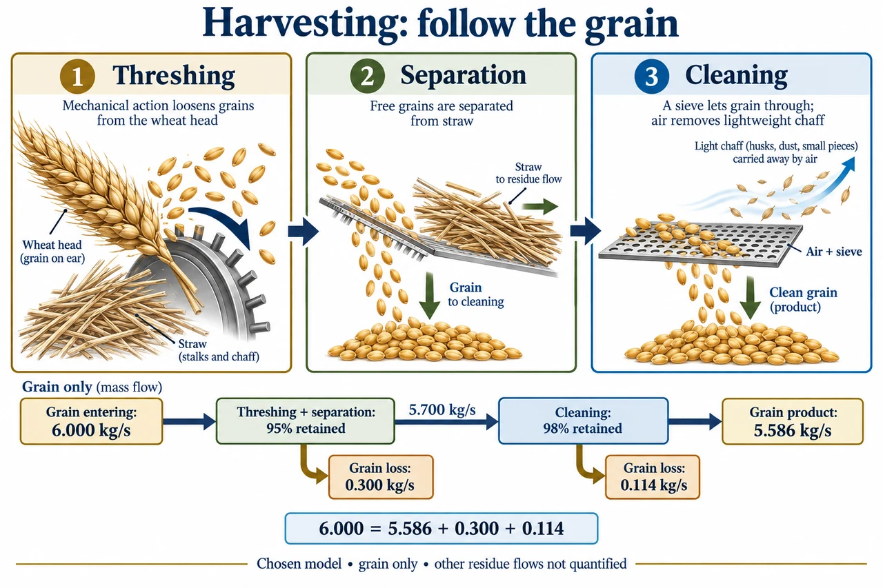
A combine harvester brings several separation jobs together, but it does not manufacture grain or turn every part of a plant into food. A crop-specific intake supplies material; threshing detaches grain from the structure that holds it, separation recovers loose grain from bulk residue, and cleaning removes much of the remaining unwanted material from the grain stream. The upper image panels use wheat as one symbolic example. A corn head, soybean cutterbar and wheat intake are not interchangeable universal arrangements. The drawing therefore explains process functions rather than a complete machine layout, exact header geometry or an operating procedure.

Threshing and separation are related but different. Detaching a kernel from a cob or grain from a head first requires mechanical interaction with its supporting material. Once detached, a loose grain can still remain trapped among straw or other residue. A separating stage provides opportunities for that grain to leave the bulk residue stream. Cleaning uses differences in size and response to air along with sieve passages to sort the subsequent mixture. A grain can be lost with residue or unwanted material can remain with the product; neither a visibly clean sample nor a large flow alone establishes that all incoming grain was recovered. Different crops and conditions change these responses.

The lower image deliberately tracks grain mass only. Choose a steady incoming grain rate of 6.000 kg/s after intake, with no changing accumulation in the chosen process boundary. Suppose the combined threshing and separation stages retain 95% of that grain for cleaning. Then 6.000 × 0.95 = 5.700 kg/s reaches the cleaning stage and 0.300 kg/s of grain leaves in its other output. If cleaning retains 98% of its incoming grain, product grain is 5.700 × 0.98 = 5.586 kg/s. Additional grain loss is 5.700 × 0.02 = 0.114 kg/s. The balanced account is 6.000 = 5.586 + 0.300 + 0.114. These chosen efficiencies are arithmetic assumptions, not a measured harvester rating.

Two stages retaining 95% and 98% do not together lose 5% + 2% of the original input. The second loss applies to the smaller surviving stream. Overall recovery is 0.95 × 0.98 = 0.931, or 93.1%; overall grain loss is 6.9%. At these unchanged chosen fractions, doubling grain input doubles every grain output rate but does not improve the recovery fraction. Actual fractions need not remain fixed when throughput changes. Grain damage, moisture, crop variety and material loading can affect performance, so an arithmetic extrapolation is not a capacity guarantee. Other straw and chaff flows are shown qualitatively in the top panels, not assigned invented mass rates in the lower account.

Place the boundary before blaming a stage. A count of grain behind a machine may include grain that was already on the ground before harvest, grain missed at intake, and grain from internal stages. An internal controller cannot recover pre-existing field loss simply by changing a downstream separation process. Iowa State University’s September 2026 extension account distinguishes these loss locations and the major process functions. Its earlier crop-condition discussion connects cleaning to sieve and airflow behaviour. Those mechanisms support the conceptual explanation; the source’s practical settings, historical crop forecasts and field loss rules are not transferred into this lesson as universal instructions.

Compare competing objectives explicitly. In a chosen alternative model, incoming grain rises to 8.000 kg/s but combined threshing/separation recovery is 90% and cleaning recovery 97%. Product grain becomes 8.000 × 0.90 × 0.97 = 6.984 kg/s: more product per second than 5.586, but only 87.3% recovery and 1.016 kg/s grain lost. Over a fixed 100 s operating interval, that means 698.4 kg product rather than 558.6 kg, while grain input differs. Over a fixed incoming harvest mass of 600 kg instead, the comparison is 523.8 kg recovered rather than 558.6 kg. Faster throughput and better mass recovery answer different questions. This is a model comparison, not a recommendation to operate machinery faster.

Sensing can improve feedback without making a measurement infallible. A loss sensor’s response must relate to the material and conditions it observes; a clean-grain flow sensor measures a downstream stream rather than every loss before it. A yield map also needs correct time and position association. For a fictional constant travel speed of 3 m/s, a 2 s error in assigning a delayed mass-flow observation shifts its mapped location by 6 m along travel. This elementary distance calculation does not establish any particular machine’s actual delay. The 2026 extension source notes calibration, transport delay and the need to check observations, which is why a colourful map is not itself proof of accuracy.

A useful machine assessment includes crop recovered, grain condition, energy use, residue handling, reliability, labour and access to repair. A larger machine can relieve a narrow harvest window while imposing higher purchase costs or access barriers; the preferable choice depends on the service and context. Residue can influence subsequent field conditions rather than being a meaningless waste stream. Automation should not conceal who is responsible for a misleading sensor or inaccessible repair system. The image’s gold grains and separate loss branches explain a bounded mass account; its airflow arrow identifies a physical sorting contribution, not a fan setting. Machinery guarding, fire prevention, safe access and operating adjustments require qualified guidance outside this conceptual lesson. Full family design and safety objectives remain open.

Worked example: For a chosen 10 kg/s incoming grain stream, first combined recovery is 92% and cleaning recovery 96%. Balance product and both grain-loss streams. Compare cleaning improvement to 98% with unchanged first stage. Explain what this proves and what it cannot establish about purity or operating capacity.

First survivor is 10 × 0.92 = 9.2 kg/s; first grain loss is 0.8 kg/s.

Product is 9.2 × 0.96 = 8.832 kg/s; cleaning grain loss is 9.2 × 0.04 = 0.368 kg/s. Balance: 10 = 8.832 + 0.800 + 0.368. Overall recovery is 88.32%.

At cleaning recovery 98%, product is 9.016 kg/s and cleaning loss 0.184 kg/s. Product increases by 0.184 kg/s, or 1.84 percentage points of original input; overall recovery is 90.16%.

The model accounts only for grain mass. It does not quantify impurities, damage, other plant material or the effect of changing real machine throughput.

Answer: Original product 8.832 kg/s, losses 0.800 and 0.368 kg/s. Chosen cleaning improvement gives product 9.016 kg/s, losses 0.800 and 0.184 kg/s. The balanced gain is 0.184 kg/s, not a guarantee about real machinery.

Check your understanding: Why are stage loss percentages not simply added? Can a downstream loss sensor detect every pre-harvest loss, and does more grain per second prove better recovery for a fixed incoming mass?

Answer: Later fractions act on surviving streams, so total recovery is the product of stage recoveries. A downstream sensor cannot reconstruct every earlier loss without additional evidence and a defined boundary. Larger product rate can coexist with a lower recovered fraction when incoming rate differs.

Why: Declare the grain-only boundary and steady assumptions, balance each branch, and compare like-for-like input before judging performance.