Precision agriculture: an index is not a prescription

By How things work · myAudience

myAudience original generated educational illustration · Original commissioned illustration

Precision agriculture: an index is not a prescription

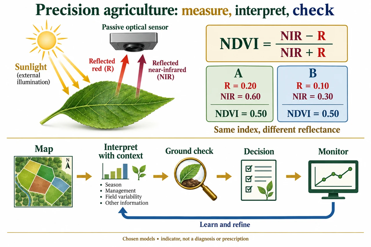
Precision agriculture connects measurements to location-specific decisions, but a map is an observation product rather than a self-explanatory prescription. A useful chain separates sensing, position and time association, interpretation, ground checking, decision-making and monitoring. The bottom of the image shows these different steps and a feedback arrow. Remote sensing is one source of evidence among others, including field observations, soil measurements and harvest records. Combining them requires compatible definitions, scales and dates. A visually striking pattern can reflect a crop, weather, sensor or processing difference without identifying a unique intervention.

The upper image describes passive optical sensing. Sunlight supplies illumination; the sensor receives some light reflected from the surface. The red and near-infrared rays drawn upwards from the leaf are reflected radiation, not a sensor illuminating the leaf and not the plant’s thermal emission. Chlorophyll absorption contributes to relatively low red reflectance, while leaf structure influences near-infrared scattering. The proportions also depend on background, geometry and conditions. A single leaf cartoon is not a complete canopy model. NASA’s historical vegetation explanation supports this mechanism, while its old instrument-development outlook is not treated as a current technology ranking.

One widely used summary is NDVI = (NIR − R)/(NIR + R), using compatible near-infrared and red reflectance measurements with a nonzero denominator. USGS describes its Landsat products as derived from processed surface reflectance. A raw instrument count, a displayed map colour and a valid reflectance are different quantities. Stored scaled index values and fill codes also require their product definition; a missing observation must not be interpreted as an unusually stressed crop. Band numbering differs between instruments, so the algebra uses physical bands rather than claiming that one band number works everywhere.

The image compares chosen reflectance pairs, not actual crop observations. Pair A has R = 0.20 and NIR = 0.60, giving (0.60 − 0.20)/(0.60 + 0.20) = 0.50. Pair B has R = 0.10 and NIR = 0.30, giving 0.20/0.40 = 0.50 as well. The two bands have both halved, but the index has not changed. More generally a positive common multiplier cancels from the ratio. NDVI therefore discards some brightness information; equal indices do not uniquely establish equal biomass, yield, water status or nutrient needs. That loss of information is part of the mathematical definition, not evidence that the instrument malfunctioned.

An additive error behaves differently. Add a chosen 0.05 offset to both channels of pair A: the reported pair becomes R = 0.25 and NIR = 0.65, giving 0.40/0.90 = 4/9, approximately 0.444. The difference numerator is unchanged but the sum denominator has grown. A common additive offset therefore does not cancel like a common multiplier. Real atmospheric correction and calibration involve more than this one arithmetic perturbation; the example demonstrates why the origin and processing of a number matter. If both valid channels were zero, the formula would be 0/0 and undefined, not an index of zero. Equal nonzero channels yield zero, which alone cannot establish that vegetation is absent.

A pixel may mix surfaces, and averaging indices is not generally the same as calculating an index from averaged bands. Choose equal-area components with vegetation R = 0.10, NIR = 0.50 and soil R = 0.20, NIR = 0.30. Their indices are 2/3 and 1/5. Under a declared simple linear reflectance-mixture assumption, the mixed bands are R = 0.15 and NIR = 0.40; NDVI is 0.25/0.55 = 5/11, about 0.455. The arithmetic mean of the two component indices is 13/30, about 0.433. They differ because the denominator changes. This chosen model is not a validated way to infer crop fraction from a real pixel, and canopy shading or multiple scattering can violate its assumptions.

Position and timing provide another uncertainty route. A downstream harvest sensor observes grain after it has travelled through a machine. If a fictional position association is wrong by 2 s at constant ground speed 3 m/s, the observation is misplaced by 6 m along travel. That can shift an apparent field boundary even when the measured flow is correct. Iowa State’s 2026 account makes the general transport-delay concern explicit; the values here are chosen, not its machine-specific delay. Repeat observations and independent ground evidence help distinguish persistent patterns from artefacts. USDA’s 2023 adoption report describes historical evidence through 2019, not the proportion of farms using these tools in 2026.

A responsible decision process asks what was measured, whether alternative causes fit, what uncertainty remains and who bears the cost of a mistake. An index alone must not automatically prescribe fertiliser, pesticide or irrigation doses. Small farms may face equipment and support costs, while shared services can introduce data-control questions. Location-tagged farm records need clear permissions and accountability; machine-learning predictions need relevant validation rather than attractive colours. The image’s two equal-index cards teach information loss, and its ground-check stage interrupts the tempting leap from map to diagnosis. No real field data, farm coordinates or individual information are used. This lesson closes a bounded ratio-and-feedback mechanism, not the family’s full agronomy, validation or environmental assessment objectives.

Worked example: Choose valid reflectances R = 0.20 and NIR = 0.50. Find NDVI, then multiply both by 1.25 and compare. Instead add 0.05 to both original channels and compare. Explain why equal NDVI is not a unique crop diagnosis.

Original NDVI = (0.50 − 0.20)/(0.50 + 0.20) = 3/7 ≈ 0.42857.

Multiplication gives R = 0.25, NIR = 0.625. NDVI = 0.375/0.875 = 3/7, unchanged.

Addition gives R = 0.25, NIR = 0.55. NDVI = 0.30/0.80 = 3/8 = 0.375, a decrease of 3/56 ≈ 0.05357.

A ratio compresses two channel values into one number. The same ratio can come from different channel magnitudes or surface mixtures, and different causes can produce similar observations. Independent context and checks remain necessary.

Answer: NDVI is 3/7 before and after common multiplication, but 3/8 after the chosen common additive offset. Neither result is a field diagnosis, dose recommendation or actual accuracy specification.

Check your understanding: For the chosen equal mixture in the prose, why is 5/11 not 13/30? Is 0/0 a valid zero index? At 3 m/s, what spatial shift follows from a 2 s association error, and is that a measured machine delay?

Answer: Calculating a ratio after mixing bands differs from averaging their separate ratios because their denominators differ. 0/0 is undefined. The chosen distance error is 6 m; it is an illustrative timing model, not an observed or universal delay.

Why: Follow physical measurement and mathematical processing separately, retain undefined/missing states, and use model assumptions rather than colour as evidence.