Air-pollution monitoring: correlation is not agreement

By How things work · myAudience

myAudience original generated educational illustration · Original commissioned illustration

Air-pollution monitoring: correlation is not agreement

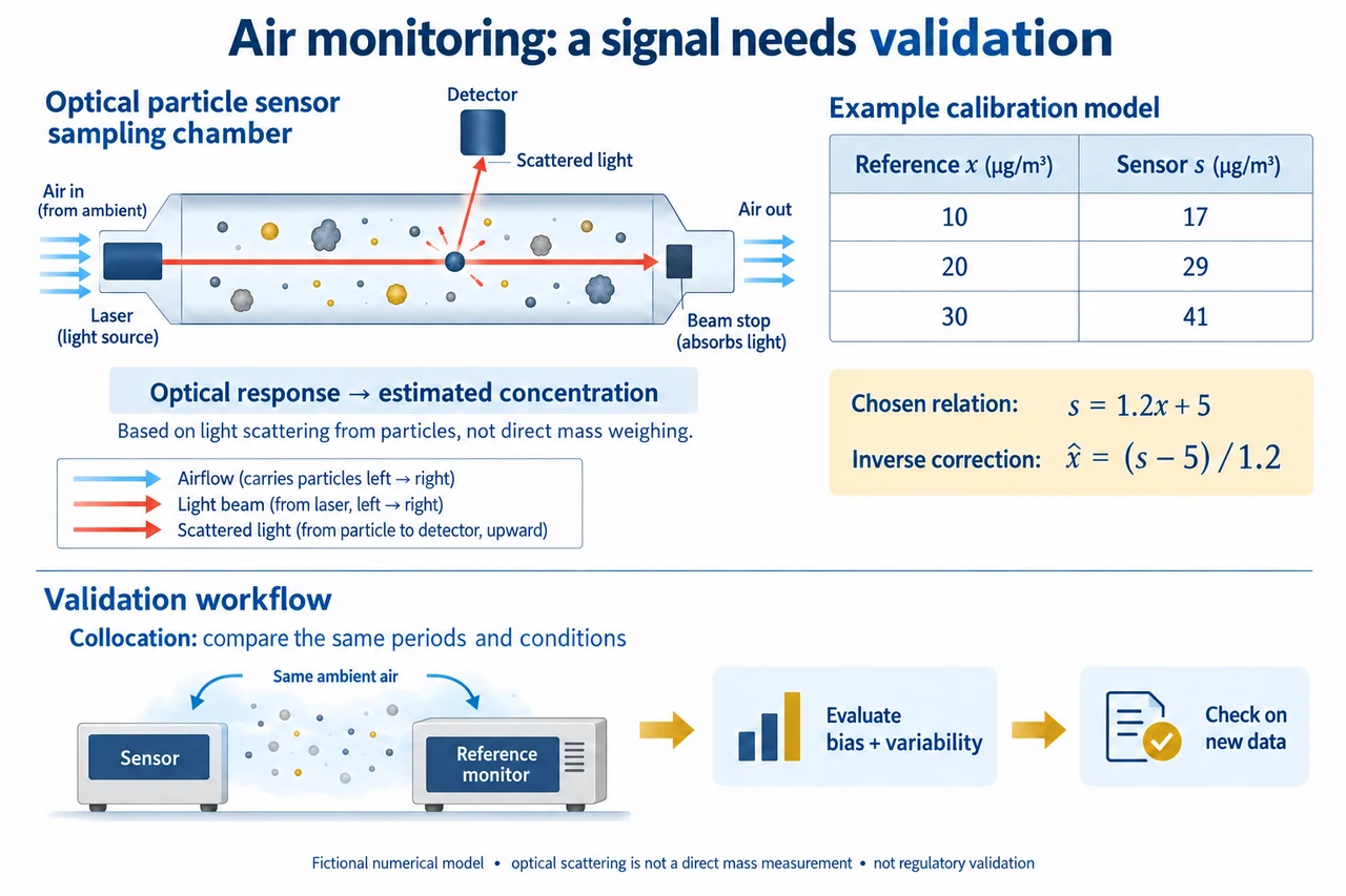
An air-pollution monitor translates a physical interaction into a reported quantity. The translation matters: a sensor reading is not the pollutant itself and not automatically a regulatory result. The image selects one optical particle-sensing mechanism, rather than claiming that the same device measures every gas and particle species. Air carries particles through a sensing region; illumination interacts with them, and a detector observes some scattered light. Electronics and a model convert that optical response into estimates such as particle count or concentration. A gas-sensitive electrochemical device uses a different interaction and cannot be substituted into this explanation without changing the mechanism.

The detector ray in the image begins at a particle and reaches the light receptor; the straight beam continues towards a beam stop while air passes through the chamber. These distinct paths must not be mistaken for a particle physically turning into an electrical signal. Scattered response depends on the particles and the measurement arrangement, so estimated mass is not a direct weighing of the sampled air. Different particle size distributions, composition and conditions can alter the relation between response and reported concentration. The symbolic layout supplies no construction dimensions, optical exposure instructions or verified sampling efficiency. It explains why a calibration relationship is needed before trusting the output.

Collocation means comparing a sensor with a suitable reference monitor under closely matched air and time conditions. EPA’s current collocation page distinguishes this comparison and mathematical data correction from changing an instrument’s settings. A reference comparison still has scope: the pollutant, concentration range, weather and time aggregation actually observed constrain what was tested. A sensor and reference reporting different averaging windows can disagree because they observed different summaries, even when both instruments are otherwise behaving consistently. The bottom image therefore places both beside the same air and calls for matched periods, followed by evaluation on new data rather than declaring universal accuracy.

The upper table is a deliberately exact fictional relationship. Choose reference values x = 10, 20 and 30 µg/m³ and corresponding sensor reports s = 17, 29 and 41 µg/m³. They satisfy s = 1.2 x + 5: the slope scales the reference response and the positive intercept contributes an offset. Errors s − x are 7, 9 and 11 µg/m³. A perfect linear association is therefore compatible with systematic disagreement. A correlation or R² value of 1 for these exact varying pairs does not make the sensor correct; agreement would also need the right scale and offset and appropriate variability. The source guidebook’s older illustrative examples are not reused as actual sensor ratings.

If that exact chosen relationship remained valid, the inverse correction is x̂ = (s − 5)/1.2. Applying it to 17, 29 and 41 gives 10, 20 and 30 respectively. Subtracting 5 without also dividing by 1.2 would leave the scale error. But matching the same three observations used to construct the relationship is only an in-sample demonstration. Choose an additional independent paired observation with reference 25 and sensor 37 µg/m³. The same correction predicts 26.667 µg/m³, leaving a positive residual of about 1.667. This does not show what caused the discrepancy; it shows that fit and evaluation are separate steps. Neither the equation nor the new pair comes from an empirical device trial.

Environmental and sampling differences can change a relationship after evaluation. EPA’s enhanced guidebook discusses humidity, temperature, pollutant mixtures and changing response over time. Those concerns motivate checking applicability rather than simply increasing the number of sensors or applying a correction derived elsewhere. Shared bias across a network does not vanish by averaging its devices. A carefully stated uncertainty account also distinguishes repeated variation from systematic mismatch and from missing observations. A concentration estimate cannot be replaced by an assumed zero just because a device stopped reporting. This lesson does not provide a calibration recipe, approved performance target or method for bypassing formal monitoring requirements.

Time aggregation can produce another avoidable error. Consider a chosen hour with concentration 10 µg/m³ for 50 minutes and 50 µg/m³ for 10 minutes. Its time-weighted mean is (10 × 50 + 50 × 10)/60 = 50/3, approximately 16.667 µg/m³. Taking the unweighted average of the two interval summaries gives 30 µg/m³, incorrectly treating them as equally long. Nor does the correct hourly mean describe the full short-duration peak or a person’s exposure history. The numerical concentrations are fictional and no health threshold or AQI category is attached to them. Current public-health interpretation must use the applicable official guidance and validated data, not this teaching model.

Community monitoring can reveal questions worth investigating, while poorly explained uncertainty can mislead or stigmatise a place. Choosing locations, making data accessible and reporting limitations affects whose experience is represented. Funding, device maintenance and support can create unequal monitoring coverage. A map linked to private locations or individual movement also needs clear permissions, and a convenient household sensor should not be presented as proof of a particular person’s health outcome. The plate’s optical pathway explains the mechanism, its fictional table demonstrates bias despite perfect association, and its final arrow requires independent checks. Full network design, pollutant chemistry, validated measurement and the family’s remaining objectives stay open.

Worked example: Choose exact paired data with sensor s = 0.8 x + 4, reference x = 10,20,30 µg/m³. Find sensor values and errors, then invert the relationship. For an independent chosen reference 25/sensor 25 pair, find corrected prediction and residual. Compute the time-weighted mean for 40 minutes at 12 and 20 minutes at 30 µg/m³, comparing an unweighted average of the interval summaries.

Sensor reports are 12,20,28 µg/m³; errors are+2,0,−2. Exact linear association still does not establish agreement.

Inverse is x̂ = (s − 4)/0.8. For independent s 25, prediction is 26.25; residual compared with reference 25 is+1.25 µg/m³.

Time-weighted mean is(12 × 40 + 30 × 20)/60 =18 µg/m³. Unweighted mean of 12 and 30 is 21, because it incorrectly treats the durations as equal.

The relationship and observations are fictional. No actual sensor accuracy, AQI classification or clinical exposure interpretation follows.

Answer: Reports 12/20/28; errors+2/0/−2. Held-out corrected value 26.25, residual+1.25. Time mean 18; unweighted interval-summary mean 21.

Check your understanding: Can perfectly correlated instruments share bias? Does applying the chosen inverse to its three training pairs prove future performance? Why is a missing report not zero, and why is particle scattering not a direct mass measurement?

Answer: Yes; association concerns co-variation, not equality of scale and offset. Fitting training pairs does not validate new conditions or observations. Missing data mean an unknown observation rather than demonstrated zero concentration. Optical response must be interpreted through particle/measurement assumptions to estimate mass.

Why: Separate physical signal, reported estimate, matched comparison, fitted correction and independent evaluation; preserve missingness and uncertainty.