District heating: keep the water and energy accounts distinct

By How things work · myAudience

myAudience original generated educational illustration · Original commissioned illustration

District heating: keep the water and energy accounts distinct

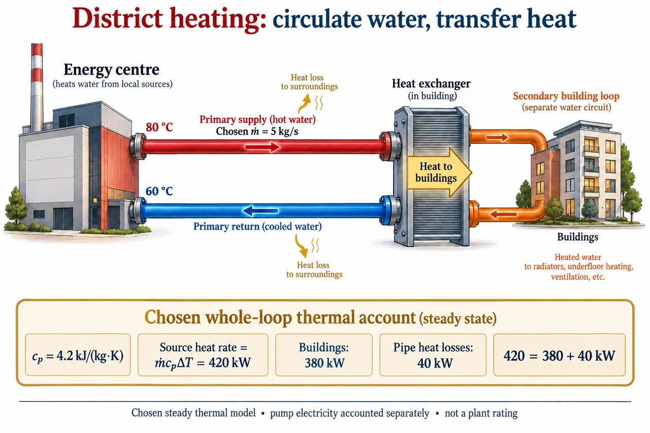
A district-heating network transfers thermal energy from one or more sources to multiple buildings through a distribution system. It can use heat from different technologies; the existence of shared pipes does not establish a particular fuel, carbon footprint or bill. The image selects a water-based indirect arrangement: primary water leaves the energy centre, transfers heat at a building interface and returns. A separate secondary building loop receives energy across the exchanger without mixing its water with the primary circuit. Direct interfaces and networks carrying steam or low-temperature heat require different details. The figure is a symbolic account, not an installation drawing or recommended operating temperature.

Follow mass and energy separately. In the selected closed primary circuit, the same water can circulate repeatedly; useful heat reaches the building while the primary water remains in its own circuit. The red arrow runs from energy centre to exchanger, and the blue return arrow runs back. Gold arrows represent heat transferred to surroundings or buildings, not water leaking from the loop. The two temperatures shown, 80 °C and 60 °C, are defined at the energy-centre supply and return boundaries. They are not also asserted as the remote exchanger’s inlet and outlet temperatures, because the drawn distribution losses can cool the water along both pipes.

For a chosen steady liquid-water model with approximately constant specific heat cₚ, thermal energy added to the circulating primary stream is Q̇_source = ṁcₚ(T_supply − T_return). Choose ṁ = 5 kg/s, cₚ = 4.2 kJ/(kg·K) and a difference of 20 K. The rate is 5 × 4.2 × 20 = 420 kJ/s, or 420 kW. A temperature difference of 20 °C corresponds to the same difference of 20 K; an absolute Celsius temperature must not be used as a Kelvin temperature in unrelated thermodynamic formulas. The constant cₚ is a chosen approximation here, not a certified fluid property across every pressure or composition.

The lower account allocates this chosen thermal rate to 380 kW delivered to buildings and 40 kW lost through distribution: 420 = 380 + 40 kW. Over one hour at those unchanged rates, the corresponding energies are 420, 380 and 40 kWh. No heat is silently lost from conservation; it is transferred to an output that is not the intended building delivery. The illustrative useful fraction is 380/420 = 19/21, about 90.48%, but that is only the chosen distribution thermal boundary. It is not the source plant’s fuel efficiency, a heat-pump coefficient of performance or a lifecycle emissions result. Pump electricity and other equipment inputs need their own declared account.

Keeping the same 420 kW thermal transport with the same chosen cₚ but reducing the supply–return difference to 10 K requires ṁ = 420/(4.2 × 10) = 10 kg/s, twice the flow. That kinematic energy balance does not by itself compute pumping power. To illustrate a separate hydraulic assumption, choose an unchanged network relationship Δp = Kq² for volume flow q and ignore changes in pump efficiency. Hydraulic power is Δpq = Kq³, so doubling q increases that model’s hydraulic power by eight. This cubic comparison is conditional, not a universal law for every pipe regime, pump or control setting. Laminar behaviour, valves and a changed network need different models.

Lower distribution losses can improve delivery without making all temperature choices interchangeable. If the model source rate remains 420 kW while pipe losses decrease to a chosen 20 kW, building delivery rises to 400 kW. If demand instead stays fixed at 380 kW, the simplified required source rate becomes 400 kW. These compare different constraints. Changing temperatures may also affect source technology and the ability of building emitters or exchangers to provide the needed service. A heat pump’s work input, for instance, cannot be omitted just because a heat source is described as waste heat. The drawing contains no heat-pump cycle or performance claim.

Actual guidance treats the network as a system to monitor and maintain. The DOE district-energy fact sheet describes thermal distribution and varied sources; its historical market figures are not reproduced as today’s totals. DESNZ’s February 2026 explanatory page discusses flow and return, interfaces, insulation, pumps and consumer concerns. Its video summaries support the concepts, but the linked videos have not been watched or adopted as operating procedures. Measurements at appropriate boundaries can distinguish generation, distribution and delivered heat. Transparent metering and explanations of losses matter because a customer should not have to guess whether an apparent efficiency gain changes their service or their bill.

A shared network can make local recovered heat available to buildings, but advantages depend on source reliability, density, access, costs and long-term care. Concentrated infrastructure can create shared outages and dependence on an operator; fairness includes understandable charges, accessible complaints and decisions about replacing assets. Environmental comparisons need the heat source, electricity and lifetime materials as well as the heat delivered. The image’s separate loops explain an indirect interface, and its lower balance prevents confusing thermal power with pumping electricity or fuel input. It claims no universally low-carbon or cheaper outcome. Full network design, consumer regulation, real performance validation and remaining family objectives remain open.

Worked example: Choose ṁ4 kg/s,cₚ4.2 kJ/(kg·K),plant-boundary supply–return difference 15 K and distribution losses 32 kW. Find source and building thermal rates and energies over 2 h. Reduce the difference to 7.5 K at unchanged source rate. Under the separate unchanged Δp=Kq² hydraulic model, compare pumping power.

Source 4 ×4.2 ×15=252 kW. Building thermal delivery 252−32=220 kW.

Over 2 h, source 504 kWh, buildings 440 kWh and loss 64 kWh. The energy balance 504=440+64 closes.

At difference 7.5 K, required mass flow 252/(4.2 ×7.5)=8 kg/s. If density is unchanged, volume flow also doubles.

Under unchanged chosen Δp=Kq², hydraulic powerKq³ becomes 8 times larger. This is a conditional hydraulic model, not a universal network rating or electricity bill.

Answer: Source 252 kW, delivery 220 kW;2-hour energies 504/440/64 kWh. Smaller difference requires 8 kg/s; selected hydraulic model gives 8 fold hydraulic power, with pump electricity still a separate account.

Check your understanding: Why are the displayed 80/60 °C temperatures at the plant rather than also at the building exchanger? Does 380/420 establish fuel efficiency, carbon savings or a household bill? Can the primary and secondary waters mix in the pictured indirect arrangement?

Answer: Distribution heat losses can change temperatures en route, so the account defines its measurement boundaries.380/420 is only the chosen useful fraction of source thermal distribution, not fuel or lifecycle efficiency or billing evidence. The illustrated exchanger transfers heat across a separating boundary while its two water circuits remain distinct.

Why: Separate mass circulation, thermal rate, energy over time, hydraulic work, source performance and consumer service before claiming an outcome.