Graphene: structure, sheet resistance and the finished device

By How things work · myAudience

myAudience original generated educational illustration · Original commissioned illustration

Graphene: structure, sheet resistance and the finished device

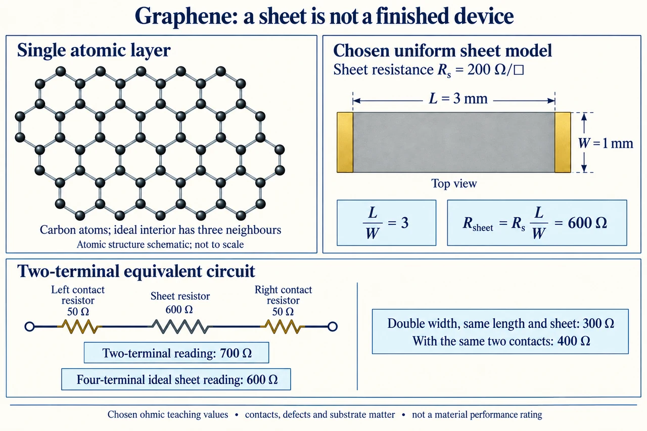
Graphene is a single atomic layer of carbon arranged in a honeycomb network. The lattice panel shows carbon at the vertices, with three neighbours for an ideal interior atom; boundary atoms have fewer depicted neighbours because the patch stops. It is neither a collection of hexagonal molecules floating separately nor a three-dimensional diamond network. Three in-plane bonding directions support the sheet, while the electronic structure permits charge transport across it. The atomic drawing and millimetre strip depict different scales and must not be overlaid as a calibrated magnification. Stacking layers, changing their relative orientation, adding chemical groups or dispersing flakes in a polymer produces a different material system whose performance requires its own evidence.

A strong in-plane bond does not by itself prove that a macroscopic product is unbreakable, and mobile charge carriers do not make a sheet a zero-resistance wire. Electrical transport depends on carrier population, scattering, geometry, temperature and interfaces. NIST atomic-scale investigations show why defects and the underlying substrate belong in the mechanism rather than only in a footnote. A substrate can produce spatial variations in carrier density; lattice defects can scatter charge carriers. A useful characterisation therefore asks what was made, where it was measured and under what conditions. The ideal lattice is a starting model, not a certificate for an unknown batch or finished device.

To separate material response from shape, consider an original uniform, isotropic, ohmic sheet model at a fixed temperature and carrier state. Conventional bulk resistance is R = ρL/(Wt), where ρ is resistivity, L length, W width and t thickness. Defining sheet resistance Rₛ = ρ/t gives R_sheet = Rₛ L/W. For an atomic sheet, sheet resistance is often a more useful directly measured description than assigning an ambiguous effective bulk thickness and quoting a bulk resistivity. The symbol Ω/□ means ohms per square: L/W is dimensionless, and a square sample has one square regardless of its absolute side length. It does not mean dividing resistance by square metres. Nonuniform, ballistic or strongly geometry-dependent samples require a model beyond this simple relation.

The plate deliberately chooses Rₛ = 200 Ω/□, L = 3 mm and W = 1 mm. These are invented teaching values, not a specification of all graphene. There are L/W = 3 squares along the transport path, so R_sheet = 200 × 3 = 600 Ω. The gold contact bars span the width at the ends of the sheet, and L is the separation between their inner edges. If L doubles while W and sheet state remain fixed, resistance doubles; if W doubles at the same L, it halves. Making a wider path is different from improving the material. Two squares of different absolute size have the same resistance in this model, but they need not carry the same acceptable current or lose heat in the same way.

Connections introduce a second distinction. In the chosen two-terminal series equivalent, the left contact contributes 50 Ω, the sheet 600 Ω and the right contact 50 Ω, giving 700 Ω in total. A low-current, ideal four-terminal measurement senses the voltage across the sheet independently of the current-carrying contact drops; with appropriately defined sensing points it can isolate the chosen 600 Ω sheet contribution. The plate gives the ideal result without pretending to supply a real probe arrangement or a laboratory protocol. In real specimens, finite geometry, contact placement, inhomogeneity and measurement uncertainty still require corrections. A contact resistance also need not stay unchanged when a device is widened; retaining 50 Ω per contact is a stated counterfactual assumption.

Double W to 2 mm in that counterfactual while retaining L = 3 mm, Rₛ = 200 Ω/□ and both 50 Ω contacts. The sheet becomes 300 Ω and the two-terminal total becomes 400 Ω. The sheet reduction is 50%, but the total reduction is (700 − 400)/700 = 3/7, about 42.9%. At an invented 1 mA, the initial total voltage is 0.001 × 700 = 0.7 V and electrical power is I²R = 0.0007 W, or 0.7 mW; the widened total gives 0.4 V and 0.4 mW at the same current. Holding voltage constant instead would increase current when resistance falls, so it would not preserve that power comparison. The calculation describes a selected circuit boundary, not the maximum safe current of an atomic film.

A finished-device claim needs more than a clean lattice image or one good resistance reading. Ask whether the material is a continuous single layer, multilayer film, oxidised derivative or a flake network; whether defects and interfaces were characterised; whether results persist across batches, operating environments and ageing; and whether the relevant device actually performs its intended function. Established research measurements should be distinguished from proposed universal replacements for silicon or from a marketing label containing the word graphene. NIST describes contact-free microwave conductance characterisation as another measurement approach, but this lesson does not reproduce its method or claim that a microwave result automatically equals the selected direct-current circuit value. Frequency and measurement boundary matter.

Evaluate the whole decision fairly. A school choosing a touch sensor, a standards laboratory evaluating electrical traceability and a community buying a coated product have different requirements. Compare function, repairability, cost, lifetime and substantiated environmental impacts, rather than assuming a small mass of material proves a small lifecycle burden. Manufacturing workers and waste handlers also deserve material-form-specific exposure assessment; no DIY synthesis, powder handling or disposal procedure is supplied here. An evidence-based procurement statement would name the tested device, conditions, uncertainty and relevant alternatives. An ethical correction withdraws an unsupported universal claim while retaining the genuine scientific achievement: atomic structure can enable distinctive behaviour, yet geometry, interfaces and the surrounding system decide useful performance.

Worked example: A fictional uniform film has Rₛ = 120 Ω/□, L = 4 mm and W = 2 mm, with two contacts of 30 Ω each. Find sheet and two-terminal resistance. Then double width with unchanged sheet state and contacts. Compare sheet and total percentage reductions, and total power at a fixed 2 mA. Explain why keeping voltage fixed changes the comparison.

L/W = 2, so sheet resistance = 120 × 2 = 240 Ω. Add contacts: total = 240 + 30 + 30 = 300 Ω.

W = 4 mm gives one square and sheet 120 Ω. The stated contacts give total180 Ω. Sheet reduction50%; total reduction120/300 = 40%.

At 2 mA, initial power = (0.002)² × 300 = 0.0012 W = 1.2 mW; widened total gives 0.72 mW. Voltage drops are 0.6 V and 0.36 V respectively.

With the initial 0.6 V held constant instead, current rises from 2 mA to 0.6/180 A ≈ 3.33 mA and total power becomes 0.6²/180 = 0.002 W = 2 mW. This is a different constraint, not a contradiction.

Answer: Sheet 240→120 Ω; total 300→180 Ω; 50% versus 40% reduction. Fixed-current power 1.2→0.72 mW, whereas fixed 0.6 V power 1.2→2 mW.

Check your understanding: A seller reports a two-terminal resistance of400 Ω for a graphene strip. Can this number alone establish its sheet resistance, layer count, defect density, durability or superiority over another material? Why is Ω/□ not Ω/m²?

Answer: No. Geometry, contact contribution, material form, measurement conditions and uncertainty are missing. If the selected model and all quantities were known, Rₛ = (R_total − R_left − R_right)W/L; otherwise many different sheets and contacts can produce400 Ω. Ω/□ labels a dimensionless aspect-ratio count, not an area-normalised resistance. Layer count and durability need separate evidence.

Why: Separate atomic structure, sheet response, geometry, interfaces and the device-level claim; apply the chosen model only where its assumptions hold.