Why a loaded generator needs more shaft work

By How things work · myAudience

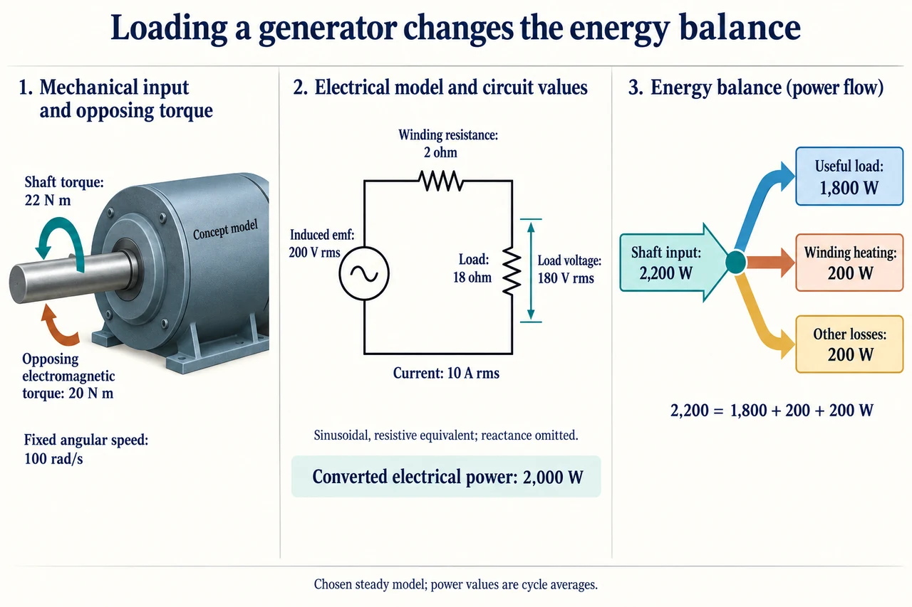
myAudience original rendered teaching illustration. Image: illustration, not a documentary photograph. · Operator-authored generated illustration; scientific model reviewed separately.

Why a loaded generator needs more shaft work

A generator’s induced emf, its terminal voltage and the power received by a load are three related quantities. They are not interchangeable labels for “how much electricity” is made. Begin by declaring the boundary: mechanical work enters through a shaft, useful electrical power leaves through the load terminals, and dissipation occurs inside the machine. We will analyse a deliberately reduced, sinusoidal resistive equivalent with fixed rotation speed and fixed induced emf. It omits reactance, excitation control, magnetic saturation and changing resistance with temperature. Those omissions make the reasoning inspectable; they prevent using the result as a real generator rating. The existing introductory cutaway explains the context, while this plate supplies a distinct circuit and accounted power model.

For a simple N-turn rotating loop in a uniform magnetic field, choose the angle θ between the field and the loop’s area normal. Flux through one turn is Φ = BA cos θ. At constant angular speed ω, θ = ωt and Faraday’s law gives e(t) = −N dΦ/dt = NABω sin(ωt). The peak induced emf is therefore NABω. Flux is greatest when the area normal aligns with the field, but the instantaneous emf is then zero because the flux is momentarily not changing. Confusing the largest flux with the largest emf reverses the mechanism. This derivation is one rotating-loop model, not an assertion that every industrial generator has rotating copper windings. Pole count, field arrangements and control must be considered before relating a real shaft speed to electrical frequency.

A sinusoid has zero signed mean voltage over a complete cycle, yet can deliver positive average power to a resistor. Voltage and current reverse together, so their product does not average to zero. Define the rms value as the square root of the time-mean square: for a sinusoid E_rms = E_peak/√2. A chosen 200 V rms induced emf thus has approximately 282.8 V peak. All circuit currents and voltages labelled on the plate are rms values; all powers are cycle averages. For a purely resistive load, average power is I_rms²R. Applying that equation to a peak current without the factor from averaging would double the answer. Reactive circuits require phase information, so a general AC load cannot automatically be analysed as this resistor.

Trace the centre circuit as one closed series loop. The chosen induced emf is 200 V rms, the winding resistance R_w is 2 Ω, and the load resistance R_L is 18 Ω. Current is I = E/(R_w + R_L) = 200/20 = 10 A rms. The winding voltage drop is 20 V rms and the load voltage is 180 V rms. The voltage bracket spans only the load; 200 V is not its terminal voltage. Load power is 10² × 18 = 1,800 W; winding heating is 10² × 2 = 200 W. Their sum is the converted electrical power EI = 2,000 W. These invented values are internally consistent assumptions, not observations from the housing artwork.

Connecting that load requires additional mechanical work. Lenz’s law opposes the change driving induction, rather than promising that every induced magnetic field points opposite every existing field. In the loaded generator, the electromagnetic interaction produces an opposing mean torque. At the chosen fixed angular speed of 100 rad/s, a converted power of 2,000 W corresponds to a mean electromagnetic torque of P/ω = 20 N m. The plate assigns a further 200 W to other losses at this operating point, giving shaft power 2,200 W and mean shaft torque 22 N m. At constant speed the input torque balances electromagnetic opposition plus the loss-equivalent torque; it does not keep accelerating the shaft. The arrows indicate opposing senses, while the housing is not a winding or pole construction diagram.

The right panel conserves energy across the declared machine-plus-load accounting: 2,200 W = 1,800 W useful load + 200 W winding heating + 200 W other losses. Do not add the 2,000 W converted-power label as a fourth output; it is the internal intermediate already partitioned into load and winding heating. Useful shaft-to-load efficiency is 1,800/2,200 ≈ 81.8%, whereas the load’s share of converted electrical power is 1,800/2,000 = 90%. Both ratios are mathematically valid and answer different questions. A claim of “90% efficient” without its boundary can conceal mechanical or magnetic losses. The chosen other-loss term may include friction, windage and core losses; it is not evidence that each mechanism consumes the same amount.

Now change only R_L to 8 Ω while the model maintains the same emf, speed and other-loss term. Current becomes 20 A, terminal voltage falls to 160 V, useful load power rises to 3,200 W, and winding heating rises to 800 W. Shaft input is 4,200 W, giving about 76.2% useful efficiency and 42 N m mean shaft torque. Doubling current quadruples winding heating; a larger power output can coincide with worse conversion efficiency. In a real machine, temperature, excitation, speed and protective limits may change, so holding these assumptions is a mathematical comparison rather than a proposal to overload hardware. Likewise the ideal result that resistive load power is greatest at R_L = R_w is not a normal safe-operating recommendation: in that limiting comparison half the converted electrical power heats the winding.

A defensible design decision starts with the service required. If the same toy model must deliver at least 180 V rms and at least 1,800 W, voltage demands R_L ≥ 18 Ω, while power is E²R_L/(R_w + R_L)². Over R_L ≥ 18 Ω this power decreases as resistance increases; only the boundary R_L = 18 Ω meets both requirements exactly. There is no margin for omitted effects. A designer should seek evidence about ratings, cooling, control response, load variation and uncertainty rather than approve a system solely because one equation reaches the target. Lower losses can reduce energy demand, but cost, repairability, material supply and the reliability needed by users remain separate judgements. State whose service is protected and what information would change the choice. Image: illustration, not a documentary photograph.

Worked example: In a different fictional sinusoidal resistive model, induced emf is240 V rms, winding resistance2 Ω, load10 Ω and other losses200 W. Speed is100 rad/s. Find current, terminal voltage, all power terms, useful efficiency and mean shaft torque. Explain why using peak current in I²R gives an error.

Series current =240/(2+10)=20 A rms; load voltage=20×10=200 V rms.

Useful load=20²×10=4,000 W; winding heating=20²×2=800 W; converted electrical power=240×20=4,800 W.

Shaft input=4,800+200=5,000 W; useful efficiency=4,000/5,000=80%; mean shaft torque=5,000/100=50 N m.

Peak current is√2×20 A; putting its square into a cycle-average I²R formula doubles every resistive power. The mean of squared sinusoid supplies the missing factor1/2.

Answer: 20 A rms,200 V rms load;4,000 W useful,800 W winding heating,200 W other losses,5,000 W shaft;80% useful efficiency and50 N m mean shaft torque. Peak-as-rms would overestimate resistive power by2×.

Check your understanding: In the200 V rms,2 Ω winding model, require at least180 V rms terminal voltage and1,800 W useful power. Find whether any R_L above18 Ω works; then explain whether reaching the boundary permits approving a real generator.

Answer: Voltage requires200R_L/(R_L+2)≥180, hence R_L≥18 Ω. Useful power40000R_L/(R_L+2)² decreases for R_L>2 Ω, so above18 Ω it is less than1,800 W; only18 Ω meets both at equality. It provides no margin and cannot certify real operation: excitation, temperature/reactance, ratings, control response and uncertainties remain omitted.

Why: For positive R_L the derivative is40000(2−R_L)/(R_L+2)³. Distinguish mathematical feasibility under declared assumptions from a measured, rated and safely controlled design.