A reliable supply needs a repair plan

By How things work · myAudience

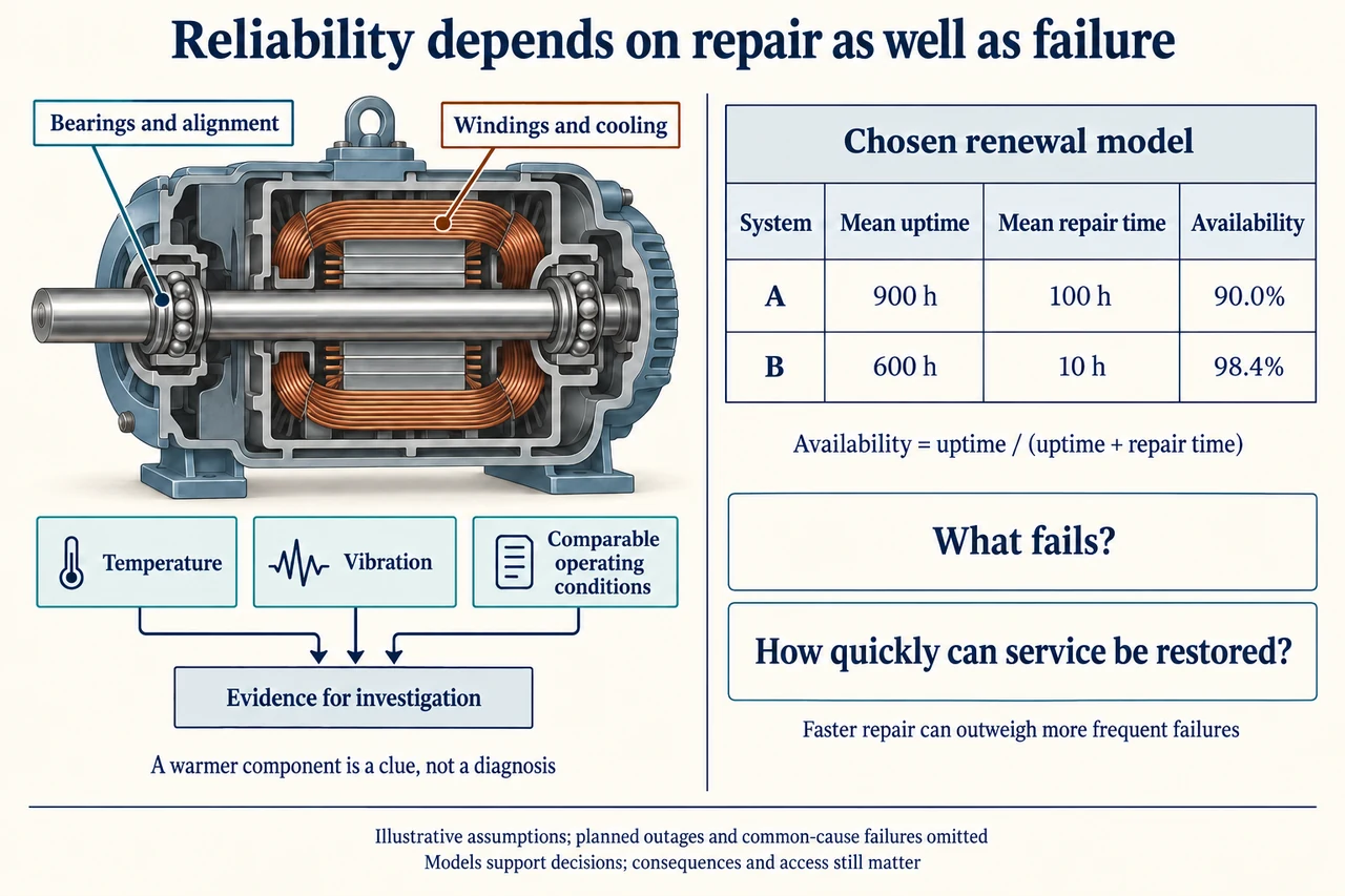
myAudience original rendered teaching illustration. Image: illustration, not a documentary photograph. · Operator-authored generated illustration; scientific model reviewed separately.

A reliable supply needs a repair plan

A generator can satisfy a power calculation and still fail to supply the service people need. Maintenance analysis therefore starts with functions and consequences: which loads depend on the machine, what counts as loss of service, and how long can the affected users tolerate interruption? Electrical conversion efficiency describes one operating condition; availability describes the share of relevant time service can be provided. Neither alone measures safety, environmental impact or affordability. The plate deliberately combines a generic component illustration with two fictional repairable-system models, not a comparison of named commercial products.

Follow the two leaders on the cutaway. Bearings support the rotating shaft, so wear, lubrication condition, alignment or imbalance can affect mechanical behaviour. The winding label identifies a different region: conductors must remain electrically separated by insulation and must transfer dissipated heat through an adequate cooling path. These materials solve different problems; a conductor with low resistance does not replace sound insulation or a correctly supported shaft. Historical Bureau of Reclamation evidence describes insulation deterioration involving thermal exposure, vibration, cracking, moisture and contamination. Its material-specific ageing examples are not universal lifetime rules for modern insulation. Inspection and interventions are professional tasks using current equipment-specific procedures, not operations to infer from this generic drawing.

The three evidence cards explain a reasoning process. A temperature change or vibration change is a reason to investigate, not a unique diagnosis. Compare records under similar loading, ambient conditions and measurement locations; a hotter reading after a larger load is not by itself proof that a bearing has worn. Several hypotheses may fit: increased losses, restricted cooling, changed load or a measurement problem. Seek a second relevant observation and the machine’s history before selecting a corrective action. DOE’s older maintenance guide distinguishes scheduled and condition-based approaches; it does not justify guaranteeing that monitoring eliminates failures. More frequent intervention can also introduce cost, downtime or damage, so “replace everything often” is not automatically the most reliable strategy.

To see why an alert is not a diagnosis, use an invented set of 100 comparable observation windows with independently established condition labels. Ten windows contain the selected degradation condition; the alert identifies eight of those ten and also flags 18 of the 90 without that condition. Sensitivity is 8/10 = 80%, but only 8/(8 + 18) ≈ 30.8% of alerts correspond to that condition. The other 72 healthy windows have no alert, and two degraded windows are missed. The two percentages use different denominators. This exercise is not a measured detector accuracy and does not prescribe an action threshold. It shows why consequences, prevalence, independent confirmation and the costs of missed versus false alerts must accompany a headline performance figure.

For the right-hand table, assume repeated operating-and-repair cycles with finite mean up and down times, comparable service demand and no planned outages or common-cause interruptions. Over many cycles, the up-time fraction approaches mean uptime divided by mean uptime plus mean repair time. System A has chosen means of 900 h up and 100 h repair: availability is 900/1,000 = 90.0%. System B has 600 h up and 10 h repair: 600/610 ≈ 98.36%, rounded to 98.4% in the table. B has a shorter mean operating interval before failure, yet higher model availability because service is restored much faster. These means are not guaranteed lifetimes, and the percentages are not probabilities that a particular new machine survives its next 1,000 h.

The repair term can include diagnosis, waiting for authorised staff or parts and restoration work, depending on the declared data definition. A distant service network may therefore dominate availability even if the device itself is well made. Conversely, comparing a hands-on repair duration for one product with a full restoration delay for another is unfair. Failure rates can change with age and operating conditions; a single constant mean can hide early failures or wear-out. Redundancy does not solve this automatically: two machines sharing the same fuel, cooling or control weakness can fail together. An independent two-unit model cannot be used if those common causes matter. Record the missing dependencies before translating a model percentage into a service promise.

In an invented steady planning window of 1,000 h, suppose either system serves a constant 20 kW demand when available, with no alternate supply. Expected unserved energy under these assumptions is 20 × 1,000 × (1 − availability). A gives 2,000 kWh; B gives about 327.9 kWh, a difference of about 1,672.1 kWh. These are model expectations, not a guaranteed calendar outage schedule. If interruptions happen when demand is low, this constant-demand model overstates the burden; if a short interruption spoils a process or affects vulnerable users, energy alone understates consequences. Do not treat every missing kilowatt-hour as equally harmful or convert health and safety into an unexplained monetary score.

Finally compare lifecycle commitments rather than only purchase price. Use fictional capital costs of 7,000 currency units for A and 10,000 for B, annual upkeep of 500 and 900, and the same 1,000 h planning window each year for four years. With a chosen unserved-energy accounting charge of 2 units/kWh, no discounting and all other costs equal, total A cost is 25,000 units; B is about 16,223. The charge is a declared scenario value, not a universal price on interruption. At zero charge A is cheaper; the break-even charge is about 0.688 units/kWh. A community could reasonably reject that narrow ranking because safety, accessible repair training, local pollution, waste and distribution of service matter. Explain the alternative, missing evidence and affected users’ preferences before committing resources. Image: illustration, not a documentary photograph.

Worked example: Use the two fictional systems’ exact availability fractions and lifecycle scenario above. Compare four-year costs, then find the unserved-energy accounting charge q at which their total costs match. No discounting or other unequal costs.

A unserved energy/year=20×1000×(1−900/1000)=2000 kWh. B=20×1000×(1−600/610)=20000/61≈327.869 kWh.

At q=2, A total=7000+4(500+2×2000)=25000 units; B=10000+4(900+2×20000/61)≈16222.951 units.

With symbolic q, B−A=3000+4×400−4q(2000−20000/61)=4600−(408000/61)q.

Equality gives q=4600×61/408000≈0.687745 units/kWh. Below this A is cheaper in this restricted accounting; above it B is cheaper. Other consequences are not made equal by algebra.

Answer: A25,000 units versus B≈16,223 at q=2. Break-even q≈0.688 units/kWh under the stated toy assumptions; it is not a universal social or reliability threshold.

Check your understanding: A proposed alert test has8 true positives,18 false positives,2 false negatives and72 true negatives. A salesperson calls it “80% accurate at diagnosing degradation” using sensitivity. Correct that inference, then identify evidence needed before using the availability table to promise service.

Answer: Sensitivity is8/(8+2)=80%, while the fraction of alerts corresponding to this condition is8/(8+18)≈30.8%. Those are different conditional questions; neither supplies a diagnosis by itself. Confirm condition labels, representative prevalence, costs of missed/false alerts and comparable operating conditions. For service, require clear uptime/repair definitions, variability, demand timing, support/parts delays, planned outages and common-cause dependencies; the table’s mean-based model does not guarantee a calendar result.

Why: Different denominators prevent confusing detection sensitivity with an alert’s predictive value. Separate statistical evidence, root-cause reasoning and a renewal availability assumption; none replaces safety-qualified investigation.