Use division and the factor theorem to expose roots

By UK A Level Mathematics · independent study · myAudience

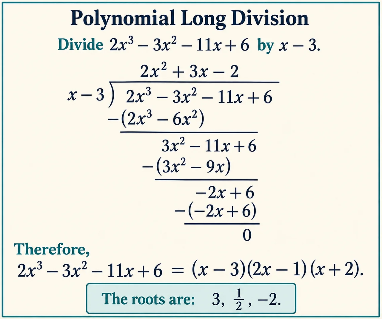
Original myAudience generated mathematics illustration; not a documentary photograph. Diagram geometry is schematic, not a calibrated measurement. · Original generated project artwork; no source textbook or exam-board figures reused.

Use division and the factor theorem to expose roots

A polynomial is a finite sum of nonnegative integer powers of a variable with coefficients. Its degree is the largest power with a nonzero coefficient. A cubic may look difficult in expanded form, but finding one linear factor reduces it to a quadratic problem. This lesson assumes confident expansion, collecting like terms and solving quadratic equations.

Polynomial division writes P(x) = D(x)Q(x) + R(x), where the remainder has smaller degree than the divisor. For a linear divisor x − a, the remainder is a constant. Substituting x = a makes the divisor term zero, giving P(a) = R. This establishes the remainder theorem and immediately gives the factor theorem: x − a is a factor exactly when P(a) = 0.

Use a suspected root to test a factor before carrying out division. If P(2) = 0, divide by x − 2 and then factor the quotient if possible. A negative root −3 corresponds to x + 3, so the sign in the factor is opposite to the root. The theorem also accommodates non-unit linear factors: a root 2/3 corresponds to 3x − 2, up to a nonzero constant multiplier.

In long division, divide leading terms, multiply back, subtract, and repeat. Write a zero coefficient for a missing power so the columns stay aligned. Subtraction applies to every term of the product you remove. Reconstruct DQ + R at the end; this checks the entire identity instead of relying on a few evaluations. The specification requires division by linear expressions here, not unrestricted higher-degree division.

Factorisation also prepares a graph sketch. A simple root usually changes the sign; a root repeated an even number of times touches the axis without changing sign. The leading term determines behaviour far to the left and right. These observations describe intercepts and end behaviour, but they do not locate every turning point of a general cubic; differentiation will supply that later.

The specialist rows show repeated cancellation of the current leading term. After subtracting 2x²(x−3), the remainder is 3x²−11x+6; after subtracting 3x(x−3), it is −2x+6; after subtracting −2(x−3), zero remains. Reconstruct the dividend by multiplying (x−3)(2x²+3x−2), which independently checks every subtraction sign. Then factor the quadratic into (2x−1)(x+2).

Transfer: find a,b such that P(x)=x³+ax²+bx+6 is divisible by both x−1 and x+2. P(1)=0 gives a+b=−7. P(−2)=0 gives 4a−2b=2. Solving gives a=−2,b=−5; P=(x−1)(x+2)(x−3). The two remainder conditions determine coefficients without doing two long divisions. A zero remainder establishes a factor; a zero quotient is a different statement.

Check the division rows by reconstructing dividend = divisor × quotient + remainder. This equality supplies a stronger check than copying the algorithm; the remainder must have smaller degree than the divisor.

Worked example: Factor P(x) = 2x³ − 3x² − 11x + 6 given that x = 3 is a root.

P(3) = 54 − 27 − 33 + 6 = 0, so x − 3 is a factor.

Division gives quotient 2x² + 3x − 2 and zero remainder.

Factor the quotient as (2x − 1)(x + 2).

Answer: P(x) = (x − 3)(2x − 1)(x + 2); roots 3, 1/2, −2.

Check your understanding: What is the remainder when x³ − 2x + 5 is divided by x + 1?

Answer: 6.

Why: The divisor vanishes at −1. Substitution gives −1 + 2 + 5 = 6; therefore x + 1 is not a factor.