Track coordinates through graph transformations

By UK A Level Mathematics · independent study · myAudience

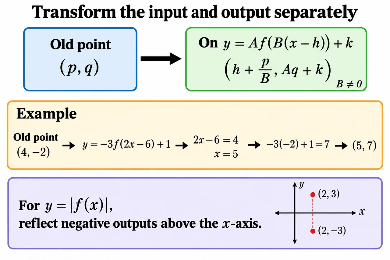
Original myAudience generated mathematics illustration; not a documentary photograph. Diagram geometry is schematic, not a calibrated measurement. · Original generated project artwork; no source textbook or exam-board figures reused.

Track coordinates through graph transformations

Graph transformations change a whole input–output relationship. If (p, q) lies on y = f(x), then (p, aq) lies on y = af(x), and (p, q + a) lies on y = f(x) + a. These are changes to the output coordinate. A negative multiplier reflects across the x-axis as well as scaling. This lesson includes combinations, which extend beyond the individual transformations in AS section 2.8.

An inside change acts on inputs. On y = f(x + a), the old input p is reached when x = p − a, so (p, q) moves to (p − a, q). On y = f(ax), with a ≠ 0, the old input is reached at x = p/a. Thus multiplying the argument by 3 compresses horizontal distances to a third; it does not stretch them by 3. The point rule explains the apparently reversed direction.

For y = A f(B(x − h)) + k with B ≠ 0, solve B(x − h) = p to obtain x = h + p/B. The point becomes (h + p/B, Aq + k). This single calculation prevents confusion about transformation order. In particular, f(2x − 6) is f(2(x − 3)), so its horizontal shift is 3, not 6. Expressions that look similar can encode different shifts.

Apply the same coordinate rule to the domain and important features. A vertical asymptote at old input p maps to x = h + p/B; a horizontal asymptote at old output q maps to y = Aq + k. When B is negative, interval endpoints reverse order and should be rewritten in increasing order. An output shift can change which points are x-intercepts, so do not carry old roots across without adjusting the output.

The rule works for quadratics, cubics, quartics and reciprocal functions already encountered. It will also work for trigonometric and exponential functions once their base graphs are known. Those families and their transformations remain pending here. For an unfamiliar given graph, use several labelled points and any asymptotes to explain your sketch rather than relying on a remembered picture.

Suppose f is defined only for 1≤u≤5 and a point (4,−2) lies on it. For H(x)=−3f(2x−6)+1, solving u=2x−6 gives x=3+u/2. Thus the domain is 7/2≤x≤11/2 and the point becomes (5,7). The coefficient 2 inside f compresses horizontal distances by one half; −3 outside reflects and triples vertical distances before adding 1.

Transfer: K(x)=f(6−2x). The inequalities 1≤6−2x≤5 give 1/2≤x≤5/2 after reversing inequalities when dividing by −2. The point's input 4 becomes x=1, with unchanged height −2. Reflection reverses the domain endpoints' order. Transform each endpoint or solve the inequalities; multiplying the old interval by −2 is not the input transformation.

Track a single known input-output pair through each transformation in the illustration. Horizontal changes act on the input and therefore require solving for the new input; do not copy the direction used for vertical translations.

Worked example: A point (4, −2) lies on f. Where does it move on y = −3f(2x − 6) + 1?

Solve 2x − 6 = 4, so x = 5.

Transform the output: y = −3(−2) + 1 = 7.

Answer: (5, 7).

Check your understanding: Where is the vertex of y = 2(x + 4)² − 3?

Answer: (−4, −3).

Why: The base vertex (0, 0) shifts left four and down three. The factor 2 changes height away from the vertex.