Solar power: rating, temperature and the hours that matter

By How things work · myAudience

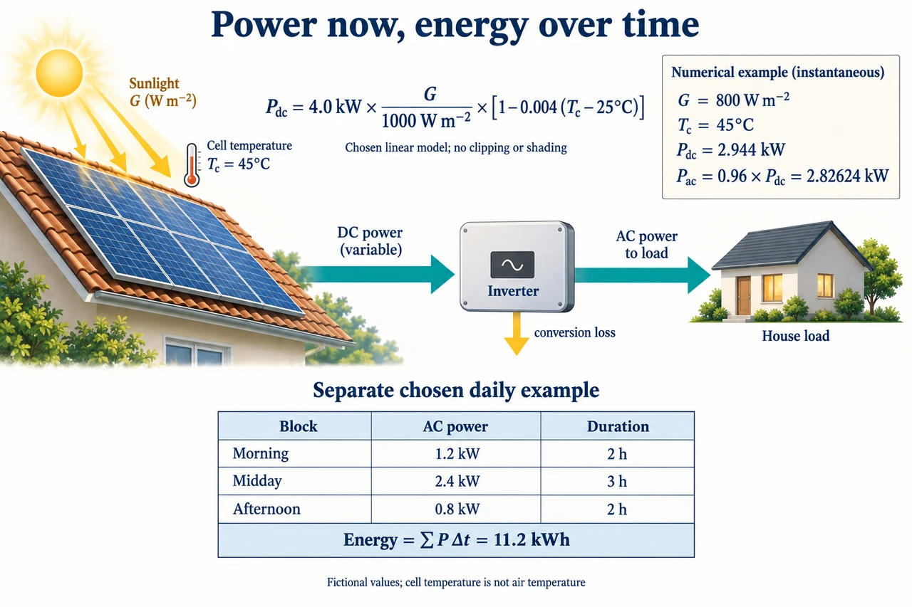
myAudience original rendered teaching illustration. Image: illustration, not a documentary photograph. · Operator-authored generated illustration; scientific acceptance reviewed separately.

Solar power: rating, temperature and the hours that matter

A solar module's nameplate is a comparison under specified test conditions, not a promise of that power throughout the day. Irradiance is incident radiant power per unit area, measured in W/m²; irradiation is the time-integrated energy per area. The relevant surface is the plane of the module, not automatically a horizontal weather sensor. Cell temperature describes the semiconductor's operating temperature, not the air reading. An evidence-based prediction therefore specifies orientation, time, irradiance and temperature before comparing electrical output. Under fixed reference conditions, doubling comparable module area doubles incident power and usually the available electrical scale; it does not double conversion efficiency. A 4 kW array is not a battery holding 4 kWh.

Use a deliberately reduced maximum-power model: Pdc = P 0(G/G 0)[1 + γ(Tc − T 0)], with P 0 = 4.0 kW, G 0 = 1000 W/m², T 0 = 25°C and a chosen γ =−0.004 per°C. This coefficient means a 0.4% change per Celsius degree relative to reference power at fixed irradiance within the model's limited range, not 0.4 percentage points of module efficiency per degree. G/G 0 and the temperature bracket are dimensionless. At G = 800 W/m² and Tc = 45°C, the bracket is 1 −0.004×20 = 0.92 and Pdc = 4×0.8×0.92 = 2.944 kW. The exact reduced equation resembles a documented irradiance/temperature approximation, not every stage of the current PVWatts V 8 engine. It omits spectral changes, detailed IV curves, mismatch and thermal transients; do not extrapolate until the bracket becomes negative or call it a low-light universal law.

Electrical conversion has its own boundary. If the chosen inverter converts 96% of the available DC input here, Pac = 0.96×2.944 = 2.82624 kW and its conversion loss is 0.11776 kW. That does not mean 96% of sunlight becomes AC. If a separate chosen module surface area is 20 m², incident power at 800 W/m² is 16 kW; DC efficiency is 2.944/16 = 18.4% and array-surface-to-AC efficiency is 2.82624/16 = 17.664%, before any losses excluded from the toy model. Trace the upper illustration's single DC→inverter→AC route and separate loss arrow. Arrow widths are schematic. Inverter efficiency depends on conditions, and an AC power ceiling can clip high DC power; constant 96% and no clipping are explicit assumptions, not product specifications.

Power changes over time; energy records the accumulated transfer. The lower illustration is a separate fictional day, not the upper formula sampled from weather data. Its three constant-power blocks give 1.2 kW×2 h +2.4 kW×3 h +0.8 kW×2 h = 11.2 kWh across 7 h. The time-weighted mean over those 7 h is 11.2/7 = 1.6 kW; the unweighted mean of three numbers is not the correct daily average because their durations differ. Taking the midday 2.4 kW and multiplying by all 7 h would predict 16.8 kWh, 50% above this example. Outside those chosen blocks the toy output is specified as zero for this exercise, not a statement that real systems share those hours. Integrating actual changing power requires properly timed measurements rather than selecting the brightest reading.

A load needs power when it operates, not merely an equal daily energy total. Choose a fictional 1 kW load throughout the same 7 h. Direct PV use is min(Ppv,Pload) in each block: 2 +3 +1.6 = 6.6 kWh. The unmet part is 0.4 kWh in the last block, while surplus is 0.2×2 +1.4×3 = 4.6 kWh earlier. Generation 11.2 kWh minus demand 7 kWh gives net surplus 4.2 kWh, yet the final shortfall exists because time matters. A perfect abstract store could move 0.4 kWh; a chosen 80% charging-to-delivery efficiency would require 0.5 kWh of earlier input to deliver 0.4 kWh, assuming suitable power, capacity and state of charge. This is energy accounting, not a battery design or a guarantee of an off-grid service. Grid import, curtailment and protected critical loads change the system boundary.

Uniformly reduced light and a local shadow are different experiments. Multiplying G by 0.8 could represent a chosen uniform reduction across identical independently operating modules; it does not prove 20% shaded area always means 20% lost power. Series-connected elements share current, while uneven illumination alters their IV relationships. Bypass arrangements and module-level electronics can change how a shaded section affects the available operating points; they cannot recreate light that never arrived. The plate intentionally contains no diode circuit or shaded-string prediction. A substantive next step would require the exact electrical topology, measured IV evidence and controller assumptions. Do not diagnose a real hot spot from a generic image or prescribe opening an energised module.

A fair comparison controls what changed. At the same 800 W/m², cooling the chosen cells from 45°C to 35°C changes the bracket from 0.92 to 0.96: DC power becomes 3.072 kW, an increase of 0.128 kW or 4.3478% relative to 2.944 kW. Calling this simply '4% more' confuses the difference in reference-power factor with the relative increase from the warmer baseline. A measured before/after gain cannot be attributed to temperature alone if clouds, wind, inverter limits or sensor locations also changed. Report the coefficient and uncertainty, verify calibrated timing and distinguish a model sensitivity from a demonstrated intervention. More sunlight can also warm cells, so treating temperature and irradiance as wholly independent observations requires care.

For a school or community service, compare delivered energy at useful times, repair access, payment terms and who can use the system. Rooftop ownership and upfront funds affect who receives benefits; access cannot be inferred from technical efficiency. A slightly lower annual yield may still support a valuable daytime service, while an attractive annual total may miss its evening demand. Ask which weather periods, demand patterns and outage cases are represented and whose work or land is required. A good revised choice states the objective—energy cost, resilient service, emissions or equitable access—and evidence that could reverse it. No single efficiency percentage settles those different objectives. Image: illustration, not a documentary photograph.

Worked example: Use the chosen 4.0 kW/−0.004 per°C model at 600 W/m² and 35°C, with 96% inverter efficiency. Compare to 800 W/m² and 45°C. Does a cooler cell guarantee higher power?

At 35°C the correction is 1 −0.004×10 = 0.96.

Pdc = 4×0.6×0.96 = 2.304 kW; Pac = 0.96×2.304 = 2.21184 kW.

The warmer 800 W/m² case gives 2.82624 kW AC, so the cooler case is lower by 0.6144 kW.

Cooling alone raises model output at fixed irradiance; here the irradiance changed too.

Answer: 2.21184 kW AC. Cooler cells do not guarantee larger total power when incident irradiance is lower.

Check your understanding: A claim says 11.2 kWh solar output is enough for 1 kW throughout the 7 chosen hours, without storage or imports. Correct it and determine the idealised storage input needed to cover the mismatch with 80% end-to-end efficiency.

Answer: Direct service is 6.6 kWh and unmet demand 0.4 kWh. Earlier surplus 4.6 kWh exists. Delivering 0.4 kWh with 80% end-to-end efficiency needs 0.5 kWh earlier input, plus adequate power/capacity/state of charge.

Why: Equal or excess daily energy does not guarantee simultaneity. Use minimum generation/demand per block; subtract per-block deficits, not only the daily net. Storage assumptions do not constitute real hardware sizing.