Solar lifetime: evidence, cumulative energy and responsible decisions

By How things work · myAudience

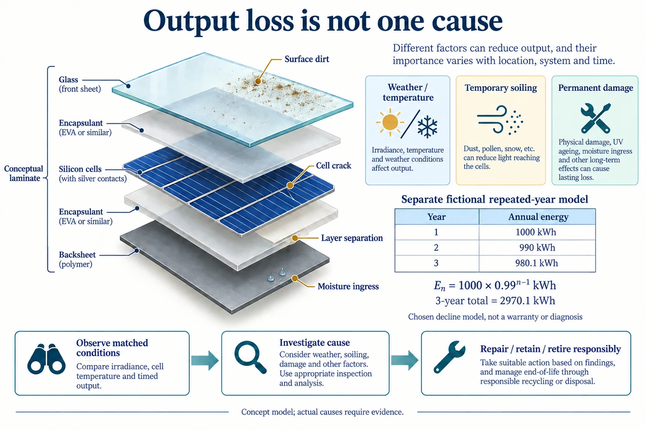
myAudience original rendered teaching illustration. Image: illustration, not a documentary photograph. · Operator-authored generated illustration; scientific acceptance reviewed separately.

Solar lifetime: evidence, cumulative energy and responsible decisions

A lower output reading does not identify a cause. Clouds or hotter cells can temporarily reduce available power; surface deposits can reduce incoming light; cracks, corrosion or separated layers may change the module itself. An inverter outage or missing data can also lower recorded system energy without proving solar-cell degradation. The illustration separates weather, reversible soiling and lasting damage rather than presenting every loss as ageing. Its exploded laminate is one simplified silicon-module construction with protective glass, encapsulation, cells and backsheet; other products use different rear materials and architectures. The callouts illustrate possible mechanisms, not a diagnosis of the pictured healthy array or a fabrication specification.

The measurement boundary determines what a trend means. Compare a module's electrical performance under matched irradiance and cell temperature before claiming a change in conversion behaviour; compare whole-system energy with an explicit weather-normalised model before blaming modules for an inverter's downtime. Maintain the same sensor calibration, time interval and data exclusions, and report missing observations. A selected historical literature review from 2012 found a median decline of 0.5% per year across published observations, but explicitly warned that its compilation was not a scientific random sample. Surviving systems can be observed longer than failed ones, and older technologies and early light-induced changes complicate comparisons. That median is neither today's universal rate nor an individual warranty; our separate 1% example below is chosen, not inferred from that study.

Define a repeated-year model carefully: annual energy En = E 1(1 − d)^(n −1), with E 1 = 1000 kWh and chosen d = 0.01. Year 1 is 1000, year 2 is 990 and year 3 is 980.1 kWh. The illustration's table is exact to the shown decimals; three-year energy is 2970.1 kWh. Each 1% reduction acts on the preceding year's energy, so it is a multiplicative decline. Removing 10 kWh each year would instead give 980 kWh in year 3—a different linear model. Both can be approximations over short periods, but neither predicts a module merely because the equations are neat. Weather and demand are fixed for this hypothetical comparison; sudden failure, repairs, recovery and curtailment are deliberately absent.

The total over N years is a geometric sum: Etotal = E 1[1 − (1 − d)^N]/d for d not zero; at d = 0 it is N E 1. Derive this by multiplying the sum by(1 − d) and subtracting, leaving first term minus the term after the last. Year 20 at 1% is 1000×0.99^19, about 826.1686 kWh, while twenty-year accumulated energy isabout 18209.3062 kWh. Confusing final-year output with cumulative energy changes the question. A comparison design with fictional year 1 output 1100 kWh and d = 0.02 gives twenty-year energyabout 18281.561 kWh, despite lower year 20 outputabout 749.356 kWh. Higher early production can compensate in an unweighted cumulative total; later dependable service may still matter differently to affected users.

Choose a transparent material/energy boundary before declaring a lifecycle advantage. In an invented accounting exercise, designA requires 3000 kWh-equivalent of manufacturing and transport energy and designB requires 3600; both serve the same electrical-energy function, with no replacement, no discounting and the same comparison method. Dividing by their twenty-year delivered energy givesabout 0.164751 and 0.196919 kWh-equivalent input per delivered kWh respectively. This narrowly ranks those chosen energy inputs, not complete environmental impacts. Water, land, mining, toxicity, labour and grid displacement need separate evidence and consistent units. Adding operational maintenance or recycling energy to one option only would be unfair. If replacement is likely, its extra embodied input and recovered service must enter both sides of the accounting.

Maintenance decisions also need a counterfactual. Suppose a fictional authorised service can recover 6 kWh per day for 30 days before the next effective rain, at a billed cost of 40 currency units and a chosen value of 0.20 per delivered kWh. Recovered energy is 180 kWh, worth 36, so the narrowly financial case does not cover 40. At 0.25 per kWh it is worth 45. But the result depends on whether rain really restores performance, how quickly dirt returns and whether downtime or water costs are included. Those values are invented, not instructions to clean panels or a prediction for any climate. Safe access, material compatibility, manufacturer requirements and ecological water constraints can independently rule out a seemingly profitable action; the educational question is which evidence is missing.

End-of-service management is a chain of decisions, not a green symbol that cancels past impacts. A functioning older module may be retained, safely repaired or reused; a damaged one may need specialist retirement. Recycling can recover materials, but collection, separation, energy use, transport and usable material quality affect what is recovered. Mass recovery and functional recovery are different: recovering bulky glass does not by itself establish recovery of every small high-value or hazardous constituent. The lower plate's observe→investigate→responsible decision sequence deliberately avoids an infinite loss-free recycling loop. Accountability includes where material goes, who handles it, whether reuse has verified remaining performance and who bears costs when equipment changes owners.

A defensible choice makes uncertainties visible rather than optimising one friendly number. Families renting their homes, school staff responsible for repairs and workers handling retired material may face different burdens from investors earning energy revenue. Compare access to repair and monitoring, contract clarity, evidence of remaining service, locally meaningful impacts and how benefits are shared. If two toy models differ by less than measurement or weather uncertainty, a precise numerical ranking is weak evidence. Revise the preferred option when actual performance, repair support or disposal evidence changes. This lesson teaches transparent model comparison and material reasoning, not a universal claim that a particular technology is cheapest, most ethical or impact-free. Image: illustration, not a documentary photograph.

Worked example: For a fictional module with year 1 output 1200 kWh and a repeated 2% annual decline, calculate year 4 and cumulative years 1–4. Explain why a survey median cannot guarantee this pattern.

Year 4 = 1200×0.98³ = 1129.4304 kWh.

Years 1–4 are 1200, 1176, 1152.48 and 1129.4304 kWh.

Their sum is 4657.9104 kWh; equivalently 1200(1 −0.98⁴)/0.02.

A published distribution is a population/sample description; technology, conditions, measurement and failure/selection histories differ.

Answer: Year 4 is 1129.4304 kWh; four-year sum 4657.9104 kWh. The 2% rate is chosen, not guaranteed by a survey.

Check your understanding: In the fictional cleaning comparison, recovered energy is 6 kWh/day for 30 days and service cost 40. Derive the minimum energy value that covers that cost, then name two reasons a favourable numerical result still would not establish the right action.

Answer: Recovered energy 180 kWh; break-even value 40/180 = 2/9, about 0.222222 currency units/kWh. Safe authorised access and water/material/ecological constraints, uncertain rain/resoiling or downtime may change the action.

Why: The break-even condition equates a chosen monetary benefit with a chosen cost under fixed recovery duration. It is not a recommendation or a complete social/environmental appraisal; identify assumptions that can reverse it.