Wind power: speed, torque and the cost of a control choice

By How things work · myAudience

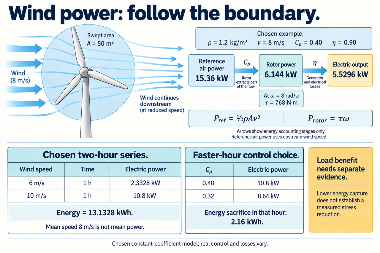
myAudience original rendered teaching illustration. Image: illustration, not a documentary photograph. · Operator-authored generated illustration; scientific acceptance reviewed separately.

Wind power: speed, torque and the cost of a control choice

A turning rotor is not yet a forecast of useful service. Start by naming three boundaries: the reference kinetic-power flux of undisturbed upstream air through the rotor's swept area, mechanical power extracted at the rotor, and electrical power delivered after the drive and generator. The swept area is a disk traced by the blade tips, not the sum of the blades' solid areas. A measurement at an unrelated height or beside a building cannot simply replace the representative upstream speed. Air density, spatial variation, direction and measurement time all affect the evidence. The existing mechanism lesson explains the shaft and generator; here the question is how a time series, rotational speed and a control choice change the conclusion.

Derive the upstream reference flux rather than memorising a cube. In a uniform undisturbed stream, a volume Av passes the reference area each second, so mass flow is ρAv. Each kilogram carries kinetic energy v²/2; their product is Pref = ρAv³/2, in watts. This is a reference denominator, not a claim that all this air keeps its upstream speed at the actual rotor. Choose ρ = 1.2 kg/m³, A = 50 m², capture coefficient Cp = 0.40 and drive-to-electric efficiency η = 0.90. These fixed coefficients are an invented limited-region model. Rotor power is Cp Pref and electric power is η Cp Pref. At v = 8 m/s the three values are 15,360 W, 6,144 W and 5,529.6 W. The plate's arrows identify these accounting stages; their widths do not measure actual airflow or electrical cables.

Rotational power adds an independently useful relationship: Pshaft = τω, where τ is torque in N m and ω is angular speed in radians per second. If the chosen 8 m/s state rotates at 8 rad/s, rotor torque is 6,144/8 = 768 N m. A generator's speed or gearbox ratio is not an energy multiplier: raising rotational speed for the same transmitted power lowers torque before losses. Choose a second operating state at 10 m/s with ω = 10 rad/s, retaining the same model coefficients. Rotor power is 12,000 W and torque 1,200 N m, while electric output is 10,800 W. In this particular proportional-speed model, power scales as v³ but torque scales as v². With real blade aerodynamics, Cp varies with rotation and pitch, so that algebra is not a universal torque curve.

Time averaging must preserve the quantity being averaged. In the plate's lower-left two-hour series, wind is 6 m/s for one hour and 10 m/s for one hour; the electrical outputs are 2,332.8 W and 10,800 W. Energy is 13.1328 kWh and mean electrical power is 6.5664 kW. Mean wind speed is 8 m/s, but calculating two hours at that speed gives only 11.0592 kWh. The actual series in this model is 18.75% above that shortcut. This follows from the curvature of v³, not from free energy or an improved efficiency. Equal interval lengths are essential to that numerical comparison. With unequal lengths, use a time-weighted speed and still compute energy interval by interval; an annual climate conclusion needs a representative measured distribution and justified operating model.

A controller changes the curve and can change the averaging error's sign. Suppose a separate fictional electrical ceiling is 12 kW. At 16 m/s the uncapped model would give 44.2368 kW, but this imposed ceiling gives 12 kW; below operating limits or during a chosen shutdown it would give zero. This arithmetic ceiling is not a physical pitch-control design or a real cut-out speed. Established controllers adjust generator torque and blade pitch to balance energy capture, operating limits and loads; specific advanced predictive or wind-farm coordination techniques remain research-dependent. A cubic extrapolation past rating is therefore invalid. Capacity factor compares energy to rated power multiplied by elapsed time; it is utilisation of a declared capacity, not conversion efficiency. State the whole elapsed window, including non-generating hours, before using it.

A measured forecast can be wrong even when the equation is correct. At unchanged coefficients and no cap, a 10% speed increase multiplies power by 1.1³ = 1.331, a 33.1% change; a first-order 3 × 10% approximation misses the higher-order terms. A 10% decrease gives 0.9³ = 0.729, a 27.1% decrease, so symmetric speed errors are not symmetric power errors. That sensitivity does not establish a probability distribution or uncertainty interval. Sensor calibration, wakes, turbulence and which height or area a reading represents are separate problems. A cloud of apparent precise watts should not obscure an unsupported speed estimate. An evidence-based revision compares timed measurements, exclusions and model residuals before assigning a cause.

Test a control trade-off under an explicit fictional choice. For the same two-hour 6/10 m/s series, option A retains Cp = 0.40 in both hours; option B deliberately reduces Cp to 0.32 only in the faster hour, retaining η = 0.90. B produces 8.64 kW in that hour and 10.9728 kWh across the two hours, sacrificing 2.16 kWh relative to A. This proves the chosen energy difference; it does not prove a percentage reduction in fatigue, because load histories and material response are missing. A responsible comparison asks what independently measured load reduction and service reliability justify that sacrifice. The lower plate separates an energy decision from the unknown load benefit, so a learner cannot infer a fatigue life merely from a reduced capture coefficient.

A community choosing dependable service needs more than a large annual number. Compare demand timing, planned and unplanned outages, network support, accessible maintenance and ecological effects with meaningful local participation. A lower output setting can be justified if well-supported evidence shows less damaging loading or valuable service continuity; it can also be unjustified if the assumed benefit never materialises. People near a project may bear noise, landscape or habitat changes while distant users receive electricity. Explain how alternatives, benefit sharing and monitored safeguards would change the decision rather than treating opposition as ignorance. Keep the air-power model, the control experiment and the social judgement distinct. Image: illustration, not a documentary photograph.

Worked example: Use the chosen ρ = 1.2 kg/m³, A = 50 m², Cp = 0.40 and η = 0.90. At 12 m/s choose ω = 12 rad/s and an imposed 12 kW electrical cap. Calculate the uncapped chain and torque; explain what the cap does not tell you about actual rotor torque.

Reference air power = 0.5 × 1.2 × 50 × 12³ = 51,840 W.

Uncapped rotor power = 0.40 × 51,840 = 20,736 W and torque = 20,736/12 = 1,728 N m.

Uncapped electrical power = 0.90 × 20,736 = 18,662.4 W; the declared output cap limits this arithmetic output to 12,000 W.

Actual controller response may change Cp, rotation, losses or curtailment. Without that response, the uncapped rotor torque cannot be claimed for the capped physical turbine.

Answer: Uncapped rotor torque 1,728 N m and electrical power 18.6624 kW; the chosen cap gives 12 kW at the output boundary only. Actual capped torque needs an additional justified control model.

Check your understanding: For the equal one-hour 6/10 m/s series, what is the energy sacrifice if only the faster-hour Cp changes from 0.40 to 0.32? Does that establish a fatigue benefit?

Answer: A gives 13.1328 kWh. B gives 2.3328 + 8.64 = 10.9728 kWh, a sacrifice of 2.16 kWh. It does not establish fatigue benefit without measured/modelled load histories and material evidence.

Why: Apply the change to the declared hour and boundary only. An energy coefficient is not a stress coefficient, damage fraction or failure probability.