Hydropower: net head, losses and the limits of an optimum

By How things work · myAudience

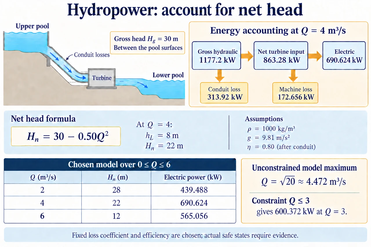
myAudience original rendered teaching illustration. Image: illustration, not a documentary photograph. · Operator-authored generated illustration; scientific acceptance reviewed separately.

Hydropower: net head, losses and the limits of an optimum

A river's flow and a dam's height are insufficient to predict electricity. A head is an energy difference per unit weight of fluid expressed as an equivalent height; elevation, pressure and speed can each contribute to it. Between large open upstream and downstream pools at similar atmospheric pressure, with surface speeds negligible, the elevation difference gives a useful gross-head approximation. Between two pipe sections, pressure and velocity terms may matter. The turbine can use only the head available at its own boundary after upstream conveyance losses. The existing mechanism lesson traces water, shaft and electrical routes; this follow-up asks when raising discharge helps, when losses reverse that trend, and what an optimisation actually proves.

Friction does not destroy energy. It reduces the organised mechanical energy available for turbine work while increasing less useful internal energy. In a steady incompressible pipe model, Darcy head loss is f(L/D)v²/(2g), with velocity v = Q/Apipe. If geometry, density and the Darcy friction factor f can be treated as fixed over a stated range, the loss is proportional to Q². Real f can change with Reynolds number and roughness; entrances, bends and screens add losses, and rapid changes need a transient analysis. Our chosen combined conduit model hL = kQ² is therefore an explicit approximation, not a universal material law or a formula for selecting a pipe. Apipe is conduit area, distinct from the turbine runner's area or a reservoir surface.

Choose gross head Hg = 30 m and k = 0.50 m/(m³/s)², with Q in m³/s. Net turbine head is Hn = 30 − 0.50Q². At Q = 4 m³/s, conduit head loss is 8 m and Hn is 22 m. With chosen water density 1,000 kg/m³ and g = 9.81 m/s², gross hydraulic power is ρgQHg = 1,177.2 kW, conduit loss power is ρgQhL = 313.92 kW and net turbine-input hydraulic power is 863.28 kW. Their equality is an energy balance across those declared boundaries. The plate separates its pool-to-pool head diagram from the accounting boxes; it is not a drawing of a particular runner or a local pressure distribution. Never subtract the same conduit loss again inside an efficiency already defined across the entire gross-head boundary.

Let the turbine-to-electric combined efficiency be a chosen constant 0.80, excluding the conduit loss just calculated. At Q = 4, electrical power is 0.80 × 863.28 = 690.624 kW and machine/conversion loss is 172.656 kW. Using gross head with 0.80 instead would claim 941.76 kW, an excess of 251.136 kW because the pipe loss was omitted. The efficiency label is inseparable from its boundary: 0.80 across net turbine input is different from electrical power divided by gross hydraulic input, which here is 690.624/1,177.2 = 0.586666…. The omitted conduit energy was not consumed by the generator and is not recoverable merely by reporting a better generator efficiency.

More discharge also creates more loss in this model. Electrical power is P(Q) = 7,848 Q(30 − 0.50Q²) watts. At Q = 2 it is 439.488 kW; at 4 it is 690.624 kW; at 6 it falls to 565.056 kW. The exact table in the lower plate illustrates those values, not a measured plant curve. The derivative measures the rate of change of power with discharge; differentiating 30Q − 0.50Q³ gives 30 − 1.50Q², so dP/dQ = 7,848(30 − 1.50Q²). Its zero is Q = √20, about 4.472136 m³/s, where net head is 20 m and power about 701.9465 kW. The second derivative is negative for positive Q, so this is the unconstrained interior maximum of the chosen equation over 0 ≤ Q ≤ 6. It is neither a real turbine selection nor an instruction to set an operating gate to that value.

A mathematical optimum is conditional on its objective and feasible set. If a fictional permit or water-allocation constraint limits turbine discharge to Q ≤ 3 m³/s, the unconstrained √20 state is unavailable. Power increases throughout the permitted range because its derivative remains positive, so the model optimum is the boundary Q = 3, giving 600.372 kW. If an electrical ceiling were 500 kW, the power-maximising output could lie on a plateau rather than uniquely at one discharge. Actual efficiency maps, cavitation limits, vibration, debris, water levels and ecological ramp constraints can remove other states. A numerical maximum with those omitted cannot be advertised as safe, legal or optimal for a real community.

A demanding sensitivity check changes the water-level assumption. Suppose downstream level rises 5 m while the upstream level stays fixed, reducing gross head from 30 to 25 m. Retain the chosen k and efficiency only for the exercise. At Q = 4, net head becomes 17 m and power is 533.664 kW, not 690.624 kW. The new unconstrained optimum is √(25/1.5), about 4.082483 m³/s, not the old √20. That comparison shows why a downstream level reading matters, but it does not prove that k and efficiency truly remain unchanged. Uncertain levels, roughness, timing and discharge measurement should enter the evidence, and a small apparent numerical advantage should not outrank uncertainty or operational restrictions.

Power is a service means, not the sole public objective. A high-output state may conflict with migration, a bypassed reach's habitat, sediment transport, domestic water supply or an acceptable rate of downstream change. Specify which people receive electricity, who has maintenance access, whose land and livelihoods are affected and which constraints are binding. Ask whether an alternative operating pattern delivers a needed service with fewer burdens, rather than ranking locations by watts alone. Existing infrastructure improvements and new impoundments have different boundaries and histories. Transparent arithmetic helps expose trade-offs; it cannot substitute for site evidence, meaningful participation or competent structural and environmental review. Image: illustration, not a documentary photograph.

Worked example: In the chosen Hg = 30 m, hL = 0.50Q², η = 0.80 model, turbine discharge is restricted to 0 ≤ Q ≤ 3 m³/s. Derive the permitted power maximum and compare it with an invalid use of gross head at Q = 3.

P(Q) = 7,848Q(30 − 0.50Q²); dP/dQ = 7,848(30 − 1.50Q²).

The derivative remains positive up to Q = 3, so the constrained maximum is at the upper boundary 3, not at the unavailable √20.

At Q = 3, Hn = 25.5 m; P = 1,000 × 9.81 × 3 × 25.5 × 0.80 = 600,372 W.

Using 30 m without conduit losses would give 706,320 W, an overestimate of 105,948 W.

Answer: Permitted maximum 600.372 kW at Q = 3 m³/s, conditional on this toy model. The gross-head shortcut overestimates by 105.948 kW.

Check your understanding: Gross head drops from 30 to 25 m while Q stays 4 m³/s. Someone multiplies the former 690.624 kW by 25/30. Is that correct when the same absolute conduit loss remains?

Answer: No. Loss is still 8 m, so net head changes from 22 to 17 m. New power is 690.624 × 17/22 = 533.664 kW; the gross-head ratio gives 575.52 kW and omits the changed loss fraction.

Why: Apply ratios across the same physical boundary. Fixed conduit loss is subtracted before the net-head conversion, and remaining assumptions must be declared.